13. Induction Motors and Two Phase Servo Motors (A)#
Objective
The purpose of this experiment is to demonstrate the operating principles of induction and two-phase servo motors. The basic parameters of a 2-phase servo motor will be measured and used to predict its torque-versus-speed characteristics for balanced operating conditions. The steady-state characteristics will be measured and compared with analytical predictions. Servo operation will be illustrated by varying the amplitude of one of the phase voltages.
13.1. Introduction#
The steady-state equivalent circuit of a 2-phase induction machine, as it will be established in Chapter 8 of ECE 32100 text, is shown in Fig. 13.1 below.
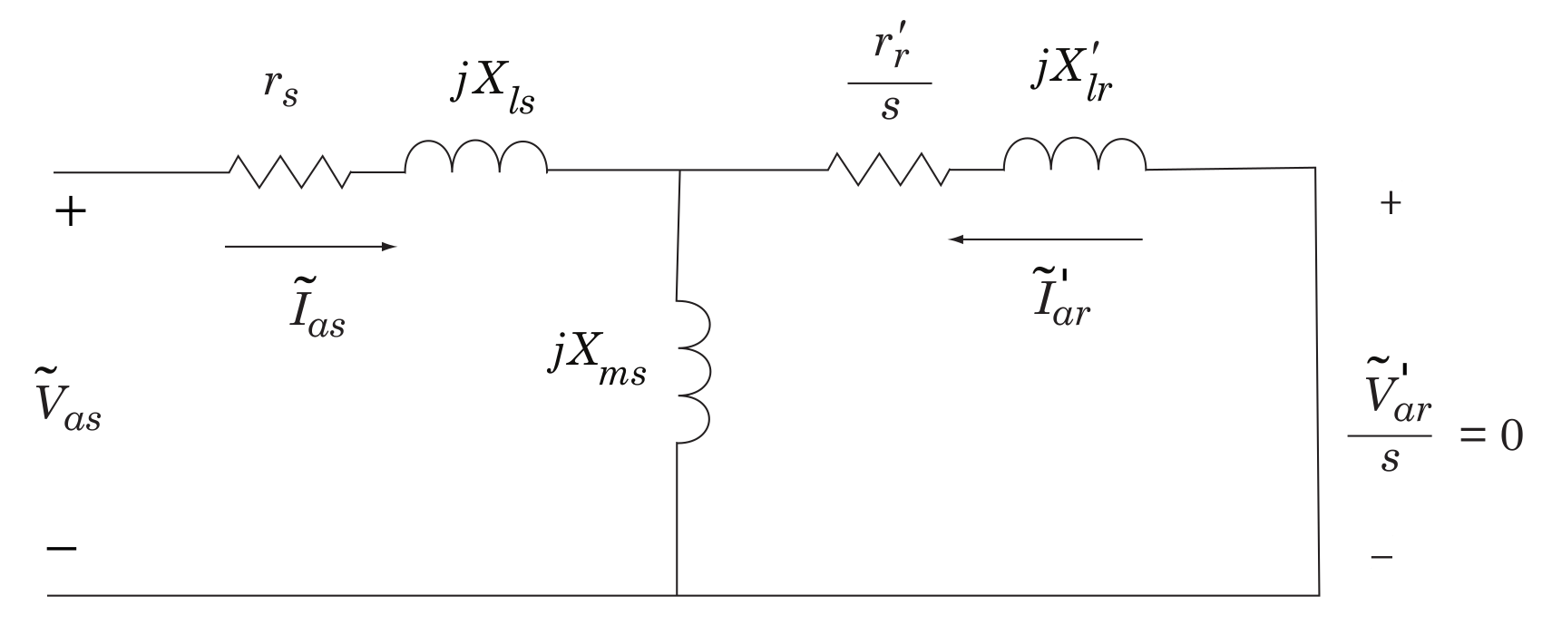
Fig. 13.1 Induction motor steady-state equivalent circuit.#
The electromagnetic torque can be expressed
With constant-amplitude constant-frequency balanced voltages applied to the stator windings
Where \(s = \dfrac{\omega_e - \omega_r}{\omega_e}\) is the slip (not to be confused with the Laplace operator).
In (13.2) and Fig. 13.1, all \(X\)’s represent \(L\)’s multiplied by the source frequency, \(X = \omega_e L\). Also,
13.2. Prelab#
Read the preceding Introduction, and subsequent In the Laboratory portions of this experiment.
13.3. In the Laboratory#
Our first objective will be to measure the electrical parameters of the motor. This can be accomplished by taking impedance measurements of the stator at stall and no-load conditions.
13.3.1. Stator Resistance#
Using the Simulink model
resistance_target.slx, apply a \(10\)-\(\V\) DC voltage to one of the AC windings. Measure the winding current.Calculate the DC resistance of the stator. This represents an approximation to \(r_s\).
13.3.2. Blocked Rotor Test#
Connect the current transducer (bottom BNC connector) outputs to Analog Input Channels 1 and 2. Set the range switch of Analog Inputs Channels 1 and 2 to \(1\). Connect the power amplifier outputs Channels 1 and 2 to the two stator phases of the induction motor.
Use the Simulink model
impedance_target.slx(Fig. 13.2) to provide a \(10\)-\(\V\) balanced 2-phase set of voltages to the stator windings connected to the power amplifier outputs, Channels 1 and 2, with a frequency of \(\qty{10}{\hertz}\).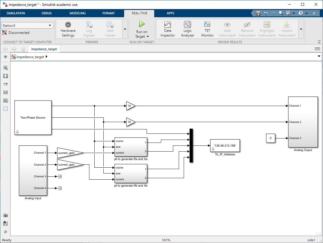
Fig. 13.2 Target model for measuring impedance.#
Prior to energizing the motor, block the rotor with your hands to prevent it from turning. With the Simulink model,
impedance_target.slx, running the on the target, open and start the Simulink modelimpedance_host.slx(Fig. 13.3). The host model will display the resistance and reactance for both the \(a\)- and \(b\)-phases. Allow the measured values to settle down (approx. \(\qty{30}{\second}\)) then flip the manual switch from \(1\) to \(0\) to record the resistance, reactance and frequency data in the MATLAB workspace. Save your MATLAB workspace by stopping the host model and typingsave lab_13_br.save lab_13_br
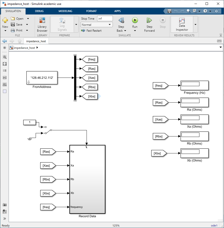
Fig. 13.3 Simulink host model for measuring impedance.#
From the equivalent circuit, the blocked-rotor impedance may be approximated as
\[(r_s + r_r^\prime) + j \omega_e ( L_{ls} + L_{lr}^\prime )\]Assuming \(L_{ls} = L_{lr}^\prime\), establish the parameters \(r_r^\prime\), \(L_{ls}\), and \(L_{lr}^\prime\).
13.3.3. No-Load Test#
Now, repeat the blocked-rotor test, using the same procedure as the blocked-rotor test, but allowing the rotor to rotate freely.
The host model will display the resistance and reactance for both the \(a\) and \(b\) phases. Remember to let the measured values settle down then flip the manual switch from \(1\) to \(0\) to record the resistance, reactance, and frequency data in the MATLAB workspace. Save your MATLAB workspace by stopping the host model and typing
save lab_13_nl.save lab_13_nl
Copy and save the file
lab_13_nl.mat. You will need this file to complete the postlab.From the steady-state equivalent circuit, the no-load impedance may be approximated as
(13.5)#\[r_s + j \omega_e ( L_{ls} + L_{ms} )\]Approximate \(L_{ms}\).
13.3.4. Blocked-Rotor Frequency Response#
Our next objective will be to calculate the frequency response of the stator.
Block the rotor with your hands to prevent it from turning.
Use the same Simulink models as used for the blocked-rotor test. Start the real-time code.
Step the frequencies from \(1\) to \(\qty{100}{\hertz}\) (using intervals \(1\), \(1.5\), \(2\), \(3\), \(4\), \(6\), \(8\), \(10\), \(15\), \(20\), \(30\), \(40\), \(60\), \(80\), \(100\)) by clicking on the 2-phase source block in
impedance_target.slx. Let the measured values settle (approx. \(\qty{30}{\second}\)). At each frequency, add the resistance, reactance, and frequency data to the workspace by flipping the manual switch from \(1\) to \(0\) inimpedance_host.slx. Save your MATLAB workspace by stopping the host model and typingsave lab_13_fr.save lab_13_fr
Copy and save the file
lab_13_fr.mat. You will need this file to complete the post lab.Plot the stator impedance as a function of frequency. Make a printout of the frequency response.
13.4. Postlab#
For the values of \(r_s\), \(L_{ls}\), \(L_{ms}\), \(L_{lr}^\prime\), and \(r_r^\prime\) established using the no-load and blocked-rotor tests, write a MATLAB script that calculates and plots the blocked rotor (\( \omega_r = 0\)) impedance versus frequency as measured from the stator, i.e.
(13.6)#\[Z = (r_s + j \omega_e L_{ls}) + (j \omega_e L_{ms}) \parallel (r_r^\prime + j \omega_e L_{lr}^\prime)\]Where the “\(\parallel\)” operator refers to the parallel combination of the two impedances. Compare this plot with measured impedance versus frequency. Explain discrepancies.
For a given frequency \(\omega_e\), why does the impedance of the motor change with rotor speed \(\omega_r\)?
How much torque will the induction motor generate with a DC input current when the rotor is stationary? How much torque is produced with a DC input current when the rotor is moving?
Plot the predicted torque-versus-speed characteristics described in (8a.2) with \(V_s = \qty{10 / \sqrt 2}{\V}\), RMS. Let \(\omega_r\) vary from \(-2 \omega_e\) to \(3 \omega_e\).
Hint
\(P=4\) and \(\omega_e = \qty{2\pi 10}{\radian\per\second}\).
At what rotor speed(s) will the electromagnetic torque be zero? Explain briefly.