Brushless DC Motor (A)

11. Brushless DC Motor (A)#

Objective

In this experiment, the rotor position of the permanent-magnet synchronous machine considered in Lab 9 and Lab 10, will be measured and used to control the frequency of a variable-frequency source (inverter). The purpose of this experiment is to show that the torque-versus-speed characteristics of the motor-inverter combination, which constitute a brushless DC motor, is similar to that of the conventional brush-type permanent-magnet DC machine.

11.1. Introduction#

The electromechanical equations of a 3-phase \(P\)-pole permanent-magnet AC machine can be expressed in the form

(11.1)#\[v_{as} = r_s i_{as} + (L_{ls} + L_{ms}) p i_{as} - \frac{1}{2} L_{ms} p i_{bs} - \frac{1}{2} L_{ms} p i_{cs} + e_{as}\]

(11.2)#\[v_{bs} = r_s i_{bs} + (L_{ls} + L_{ms}) p i_{bs} - \frac{1}{2} L_{ms} p i_{as} - \frac{1}{2} L_{ms} p i_{cs} + e_{bs}\]

(11.3)#\[v_{cs} = r_s i_{cs} + (L_{ls} + L_{ms}) p i_{cs} - \frac{1}{2} L_{ms} p i_{as} - \frac{1}{2} L_{ms} p i_{bs} + e_{cs}\]

where

(11.4)#\[e_{as} = \frac{d \lambda_{asm}}{d \theta_r} \frac{d \theta_r}{dt} = \omega_r \frac{d \lambda_{asm}}{d \theta_r}\]

(11.5)#\[e_{bs} = \frac{d \lambda_{bsm}}{d \theta_r} \frac{d \theta_r}{dt} = \omega_r \frac{d \lambda_{bsm}}{d \theta_r}\]

(11.6)#\[e_{cs} = \frac{d \lambda_{csm}}{d \theta_r} \frac{d \theta_r}{dt} = \omega_r \frac{d \lambda_{csm}}{d \theta_r}.\]

Here, \(\lambda_{asm}\), \(\lambda_{bsm}\), and \(\lambda_{csm}\) represent the flux linkages of the stator \(as\), \(bs\), and \(cs\) windings, respectively, due to the permanent-magnet rotor while \(e_{as}\), \(e_{bs}\), and \(e_{cs}\) represent the corresponding induced voltages. Also,

(11.7)#\[\theta_r = \frac{P}{2} \theta_{rm}\]

where \(\theta_r\) represents the “electrical” position of the rotor whereas \(\theta_{rm}\) represents the actual mechanical position. If \(i_{cs} = -i_{bs} -i_{bs}\), then (11.1) simplifies to

(11.8)#\[v_{as} = r_s i_{as} + (L_{ls} + \frac{3}{2} L_{ms}) p i_{as} + e_{as}\]

Equivalently,

(11.9)#\[v_{as} = r_s i_{as} + L_{ss} p i_{as} + e_{as}\]

where \(L_{ss} = L_{ls} + \frac{3}{2} L_{ms}\). Similarly,

(11.10)#\[v_{bs} = r_s i_{bs} + L_{ss} p i_{bs} + e_{bs}\]

(11.11)#\[v_{cs} = r_s i_{cs} + L_{ss} p i_{cs} + e_{cs}.\]

The electromagnetic torque may be expressed

(11.12)#\[T_e = \frac{P}{2} \left( i_{as} \frac{d \lambda_{asm}}{d \theta_r} + i_{bs} \frac{d \lambda_{bsm}}{d \theta_r} + i_{cs} \frac{d \lambda_{csm}}{d \theta_r} \right)\]

In an ideal machine,

(11.13)#\[\lambda_{asm} = \lambda_m^\prime \sin (\theta_r)\]

(11.14)#\[\lambda_{bsm} = \lambda_m^\prime \sin (\theta_r - \qty{120}{\degree})\]

(11.15)#\[\lambda_{csm} = \lambda_m^\prime \sin (\theta_r + \qty{120}{\degree}).\]

Substituting (11.13)-(11.15) into (11.12),

(11.16)#\[T_e = \frac{P}{2} \lambda_m^\prime \left[ i_{as} \cos (\theta_r) + i_{bs} \cos (\theta_r - \qty{120}{\degree}) + i_{cs} \cos (\theta_r + \qty{120}{\degree}) \right]\]

In an ideal brushless DC motor, the applied stator voltages are of the form

(11.17)#\[v_{as} = \sqrt{2} v_s \cos (\theta_r + \phi_v)\]

(11.18)#\[v_{bs} = \sqrt{2} v_s \cos (\theta_r + \phi_v - \qty{120}{\degree})\]

(11.19)#\[v_{cs} = \sqrt{2} v_s \cos (\theta_r + \phi_v + \qty{120}{\degree})\]

where \(v_s\) and \(\phi_v\) are control (input) variables. In a practical device, the applied voltages may not be true sinusoidal functions. However, we will assume that the applied voltages may be approximated as sinusoidal functions with \(v_s\) representing the RMS amplitude of the fundamental component of \(v_{as}\), \(v_{bs}\), and \(v_{cs}\).

To analyze 3-phase brushless DC machines, we define the transformation of variables

(11.20)#\[\begin{split}\begin{bmatrix} f_{qs}^r \\ f_{ds}^r \\ f_{0s} \end{bmatrix} = \frac{2}{3} \begin{bmatrix} \cos \theta_r & \cos (\theta_r - \qty{120}{\degree}) & \cos (\theta_r + \qty{120}{\degree}) \\ \sin \theta_r & \sin (\theta_r - \qty{120}{\degree}) & \sin (\theta_r + \qty{120}{\degree}) \\ \frac{1}{2} & \frac{1}{2} & \frac{1}{2} \end{bmatrix} \begin{bmatrix} f_{as} \\ f_{bs} \\ f_{cs} \end{bmatrix}\end{split}\]

where \(f=v\), \(i\), or \(\lambda\). In terms of rotor reference frame (transformed) variables, the voltage equations may be expressed

(11.21)#\[v_{qs}^r = r_s i_{qs}^r + L_{ss} p i_{qs}^r + \omega_r L_{ss} i_{ds}^r + \omega_r \lambda_m^\prime\]

(11.22)#\[v_{ds}^r = r_s i_{ds}^r + L_{ss} p i_{ds}^r - \omega_r L_{ss} i_{qs}^r\]

where

(11.23)#\[v_{qs}^r = \sqrt{2} v_s \cos (\phi_v)\]

(11.24)#\[v_{ds}^r = -\sqrt{2} v_s \sin (\phi_v).\]

Equation (11.16), when expressed in terms of transformed variables, becomes

(11.25)#\[T_e = \frac{3}{2} \frac{P}{2} \lambda_m^\prime i_{qs}^r.\]

In the steady state, \(v_{qs}^r\) and \(v_{ds}^r\) are constant. Thus, steady-state operation may be analyzed by neglecting terms proportional to \(p\) in (11.21) and (11.22) and, for notational purposes, replacing lower-case variables with upper-case variables. Solving the resulting equations for \(I_{qs}^r\) and substituting into (11.25) yields

(11.26)#\[T_e = \frac{3}{2} \frac{P}{2} \frac{r_s \lambda_m^\prime}{r_s^2 + \omega_r^2 L_{ss}^2} \left( \sqrt{2} V_s \cos \phi_v + \frac{\omega_r L_{ss}}{r_s} \sqrt{2} V_s \sin \phi_v - \omega_r \lambda_m^\prime \right).\]

11.2. Prelab#

Read the preceding introduction.

11.3. In the Laboratory#

Our first objective will be to relate the Hall-effect output voltages to the rotor position.

Caution

Never apply more than \(\qty{5}{\volt}\) to either stator winding or irreparable damage to the motor may result.

11.3.1. Hall-effect output voltages#

Hall-effect sensors are solid-state devices that can be used to detect the polarity of a magnetic field. In the given device, three Hall-effect devices are mounted on the stator of the brushless DC motor (permanent-magnet AC motor). The outputs of the Hall-effect sensors are conditioned such that when the north pole of the rotor is beneath a sensor, the corresponding output is \(\qty{5}{\volt}\). When the south pole is beneath the sensor, its output is \(0\).

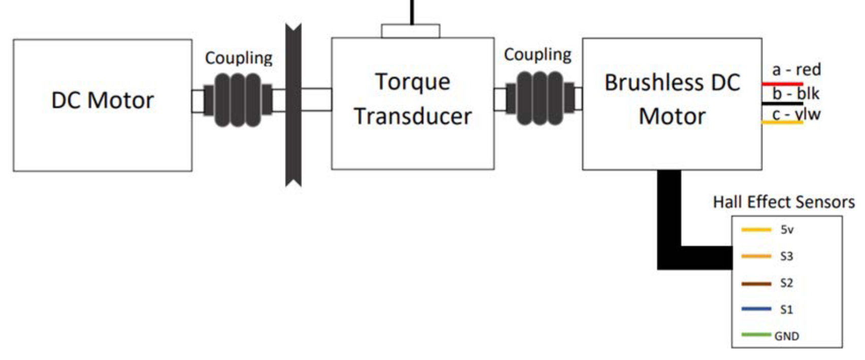
_images/setup1.png — Fig. 11.1 Experimental setup for Brushless DC Motor (A).#

Leave the stator windings of the brushless DC motor open circuited. Create a Simulink model to apply \(\qty{-5}{\volt}\) DC to the armature of the DC motor, causing both motors to rotate at a constant speed.

Note

The brushless DC motor should rotate CW when looking from the DC motor.
Using the oscilloscope, measure the output of S1 on Channel 1, the induced open-circuit voltage \(e_{ab} = v_{ab}\) on Channel 2, and the induced open-circuit voltage \(e_{cb} = v_{cb}\) on Channel 3. Determine which sensor is S1 by comparing the hall effect sensor on Channel 1 to the phase voltage on Channel 2. Measure both open-circuit voltages relative to the \(b\) phase and trigger the scope on S1.
Transfer the corresponding wave shapes to the digital computer using BenchVue. Print out the results. Store the data as phasevolt.mat.
Turn off the power to the DC motor. Leave the Channel 1 oscilloscope probe connected to Sensor 1. Connect the Channel 2 probe to Sensor 2. Connect the Channel 3 probe to Sensor 3. Again, trigger on the output voltage of Sensor 1. Reapply \(\qty{-5}{\volt}\) to the DC motor. Be sure to use the same horizontal scale on the oscilloscope as before. Transfer the corresponding wave shapes to the digital computer using BenchVue. Print out the results. Store the data pertaining to the sensors as sensor.mat.

11.3.2. Steady-state operation#

Open the model lab_11_bdc3_target.slx (Fig. 11.2 ). Build, connect to target, and start the real-time code. This program applies the appropriate voltages to the permanent-magnet AC motor such that it operates as a brushless DC motor. \(V_{DC}\) is set to \(\qty{1.0}{\volt}\). Let the motor spin up to a steady speed.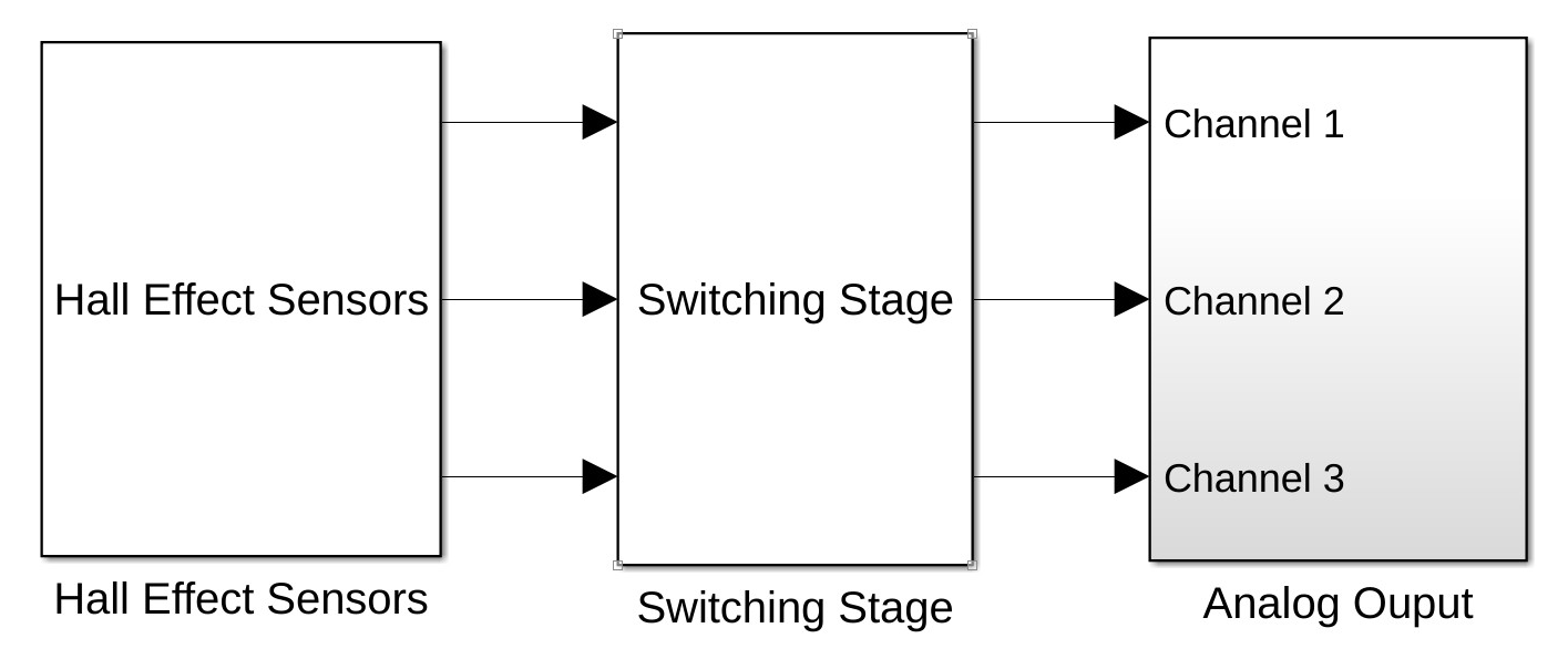

Fig. 11.2 Target model for Brushless DC Motor (A).#
Connect the three stator phase terminals to the power Channels 1, 2 and 3. In addition, connect the digital I/O cable to the digital I/O connector.
Measure the applied voltage \(v_{ag}\) (voltage from phase \(a\) to ground) and the output voltage of Hall-effect Sensor 1. Then, measure the applied voltage \(v_{bg}\) (voltage from phase \(b\) to ground) and the output voltage of Hall-effect Sensor 2. Lastly, measure the applied voltage \(v_{cg}\) (voltage from phase \(c\) to ground) and the output voltage of Hall-effect Sensor 3. What is the relationship between these voltages, the sensor outputs, and \(V_{DC}\)?

11.4. Postlab#

From MATLAB, load phasevolt.mat and sensor.mat. Calculate eas, ebs, and ecs from eab and ecb. Plot on one graph \(e_{as}\), \(e_{bs}\), and \(e_{cs}\). Plot on another graph hall1, hall2, and hall3. What was the speed of the motor?
Knowing how the applied voltages relate to the Hall sensors, calculate and plot the applied stator voltages \(v_{as}\), \(v_{bs}\), and \(v_{cs}\). Approximate these voltages as sinusoids of the form (11.17)-(11.19) by calculating their fundamental components using Fourier analysis. What is relationship between \(v_s\) and \(V_{DC}\). Plot the Hall-effect Sensor 1 voltage and \(e_{as}\) on top of one another. What is the value of \(\phi_v\)?