Introduction to Lab Experiments

1. Introduction to Lab Experiments#

Objective

The purpose of this lab session is to introduce the laboratory equipment and procedures that will be used to characterize the electromechanical devices studied in ECE 321. The main objectives are to:

Introduce the host and target computers, MATLAB/Simulink™ Real Time Workshop® (RTW), and the patch panel.
Practice acquiring, storing, and downloading waveforms using the digital oscilloscope.
Show how to load data files into MATLAB. Learn MATLAB commands to process the data.
Learn how to print oscilloscope and MATLAB graphs.
Build and run standalone Simulink models.

1.1. Introduction#

The primary focus of this lab course is to reinforce experimentally the basic principles of electromechanical energy conversion taught in ECE321 and to study the performance of different types of electromechanical devices (solenoids, motors and generators). To facilitate this learning process, the ECE323 lab has been furnished with equipment that is intended to simplify the data gathering and processing aspects of the lab. The computers used in this lab consist of a target computer (target) equipped with digital-to-analog (D/A) and analog-to-digital (A/D) converters, and a host computer (host), which is a conventional desktop PC running Windows 7 operating system and equipped with MATLAB/Simulink. This host/target computer combination serves as a signal generator, data acquisition system, signal analyzer, and print server. In this lab, we will use the computer to run a variety of packaged utilities and custom-written software.

The workstation “patch panel” is shown in Fig. 1.1 and has a variety of functions. The panel includes:

Four Analog \(+/-\) Inputs.
A 25-pin Digital Input port (For use with a position encoder).
A 9-pin Digital Input port (For use with the Hall Effect sensors on the PM Machines).
A 15-pin Digital Output port.
Three high-power analog outputs, each with two BNC connectors for voltage and current measurements. The upper BNC connector is used to measure voltage and the lower connector outputs 2 Volts per Amp flowing through the banana plugs.
Three high-power analog outputs, each with two BNC connectors for voltage and current measurements. The upper BNC connector is used to measure voltage and the lower connector outputs 2 Volts per Amp flowing through the banana plugs.

The patch panel is interfaced to the target computer using a 6-channel D/A board and a 16-channel A/D board plugged into the computer’s backplane. The digital oscilloscope has the ability to capture and store up to 4 channels of data. The oscilloscope is connected to the host computer through a universal serial bus (USB) connection.

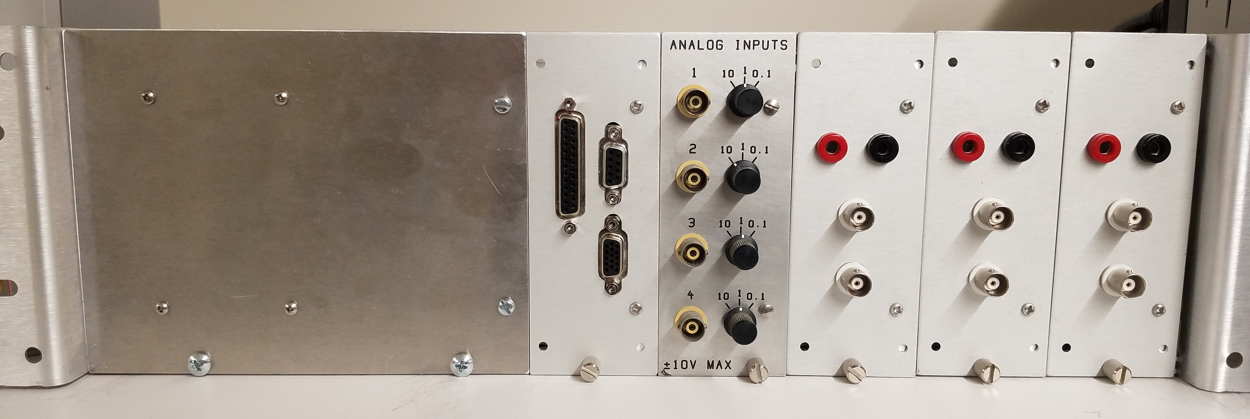
_images/fig1n.png — Fig. 1.1 Patch panel.#

In addition to the standard oscilloscope probes, this lab has been equipped with an analog torque transducer and two hall-effect current probes. The current transducers are used by simply clamping the current probe onto the wire to be monitored and connecting the Tektronix TCPA300 current amplifier output to the oscilloscope or patch panel. The torque transducer is equipped with a digital readout, but also has an analog output in the back that can be connected to the oscilloscope or patch panel.

In this course, we will use the host computer to build Simulink models and the target computer D/A outputs to generate signals to drive motors and solenoids. We will then use probes, transducers, A/D inputs, and the oscilloscope to capture and display arrays of data that are useful for characterizing the electromechanical device under study. Data captured on the oscilloscope can be downloaded to the host computer through its USB connection. The data can be displayed on the computer screen, processed using the math utilities included with MATLAB, printed on the network printer, and stored on your network account for future reference.

This first lab exercise has been prepared to familiarize you with the equipment (computers, oscilloscope, transducers, patch panel, printer, power supply), the computer programs, and the basic procedures that you will be using in future labs.

1.2. In the Laboratory#

Equipment

Computers: Host PC (Windows 7), and Target PC (Speedgoat RealTime Target)
Oscilloscope: Keysight MSOX3014T 100-Mhz Digital Storage Oscilloscope
Printer: Network HP printer
Current Transducer: Tektronix TCPA300 Current Probe Amplifier
Torque Transducer: Himmelstein MCRT transducer with 700-series Amplifier

1.2.1. Preliminary Setup (performed once at beginning of semester)#

From Brightspace, click the icon labelled Lab Files. This will download a folder labelled ECE323_Lab_Files into the downloads folder of your computer. Extract (unzip) and move this folder into C:\Users\Your Name. This folder becomes part of your ecn PC roaming profile. Navigate to the Lab1 folder in this directory. Double click the ee323lib.slx icon in the Lab1 folder to start MATLAB in the given folder (directory).
In the MATLAB command window, type slrtExplorer (Fig. 1.2). After a brief (sometimes long) delay, this will open an slrtExplorer window similar to that shown in Fig. 1.3.

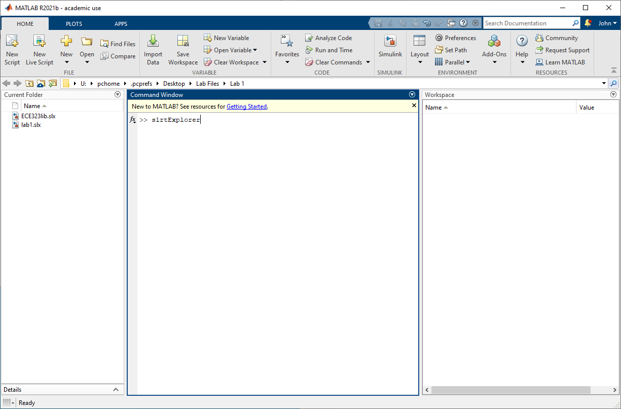
Fig. 1.2 MATLAB top-level window.#

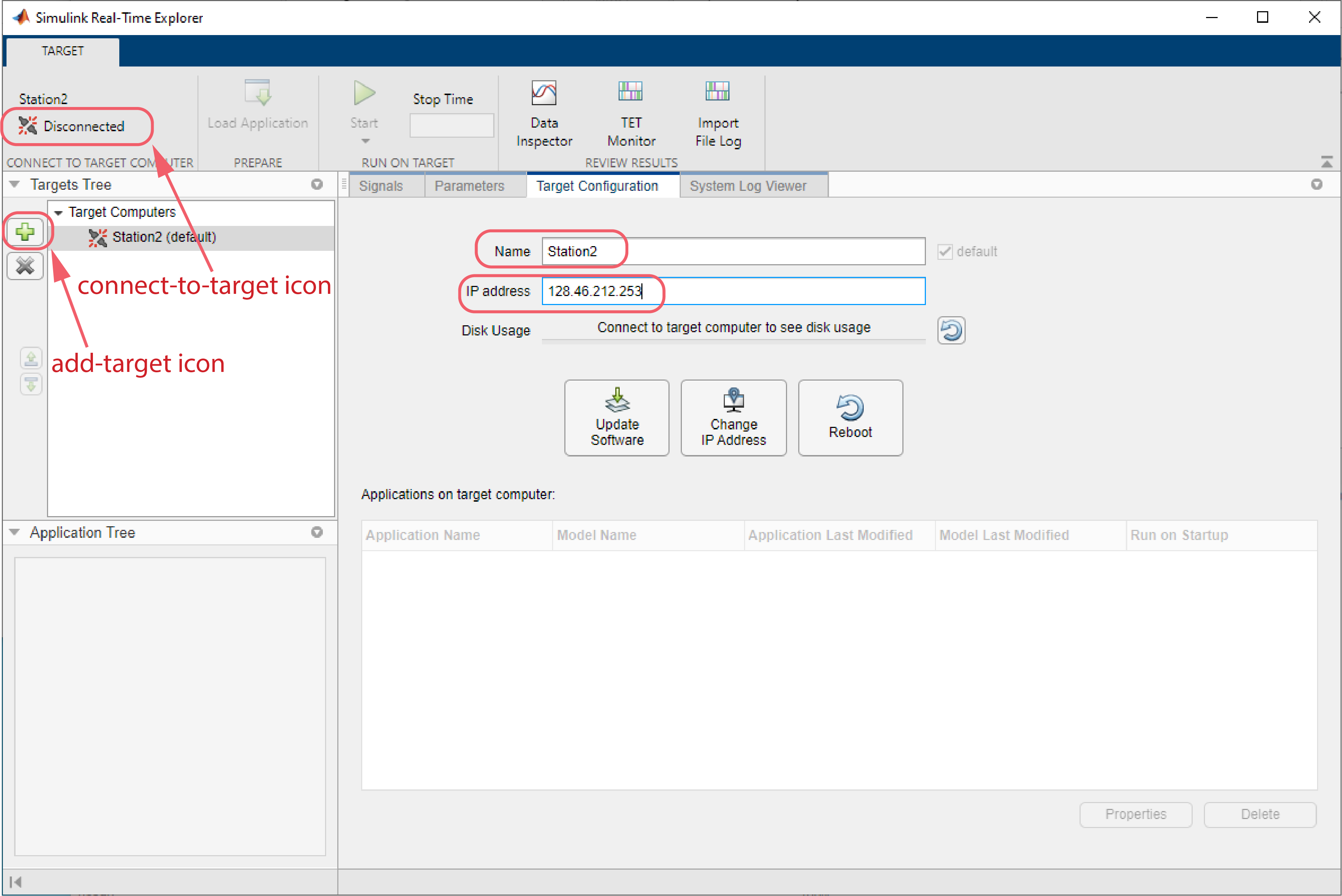
Fig. 1.3 slrtExplorer window.#

Referring to Fig. 1.3, click on add-target icon. This will create a link to a new target. Enter the name of your lab station and the IP address of the target computer in your station. Click on the Change IP Address icon. MATLAB will attempt to communicate with the target and notify you if successful. If not, see TA or instructor. Finally, click on the connect-to-target icon (Fig. 1.3), which initially displays Disconnected. The display should then change to Connected.

1.2.2. Building Target Model#

The Simulink model required to execute this experiment will consist of blocks from both the Simulink Library Browser and the ee323lib.slx file. Bring to focus the Simulink ECE323lib window (Fig. 1.4). Open the standard Simulink library by clicking the Library Browser button near the top of the window. In top left corner, select New ‣ Blank Model. This will open a blank Simulink window. Save the model window as lab1.slx.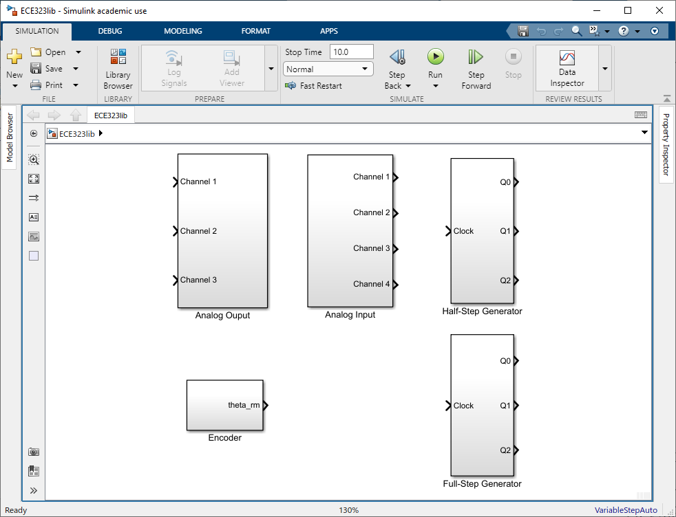

Fig. 1.4 Simulink EE323 library.#
Construction of the Simulink model begins by copying (Ctrl-C Ctrl-V) or dragging blocks from the standard Simulink library or ECE323lib to the lab1 model window. Blocks can be moved within the model by pressing left mouse button when the cursor hovers above the desired block and dragging to the desired location. In addition, when the block handles are active, they can be used to alter the size of the block. Multiple uses of the same block will result in automatic incremental labeling of the blocks. To connect the blocks, click on an arrow of one block, hold button, and drag the mouse to the termination point. Use the model blocks from the Simulink Library Browser and the ee323lib.slx file to construct the waveform generator model shown in Fig. 1.5.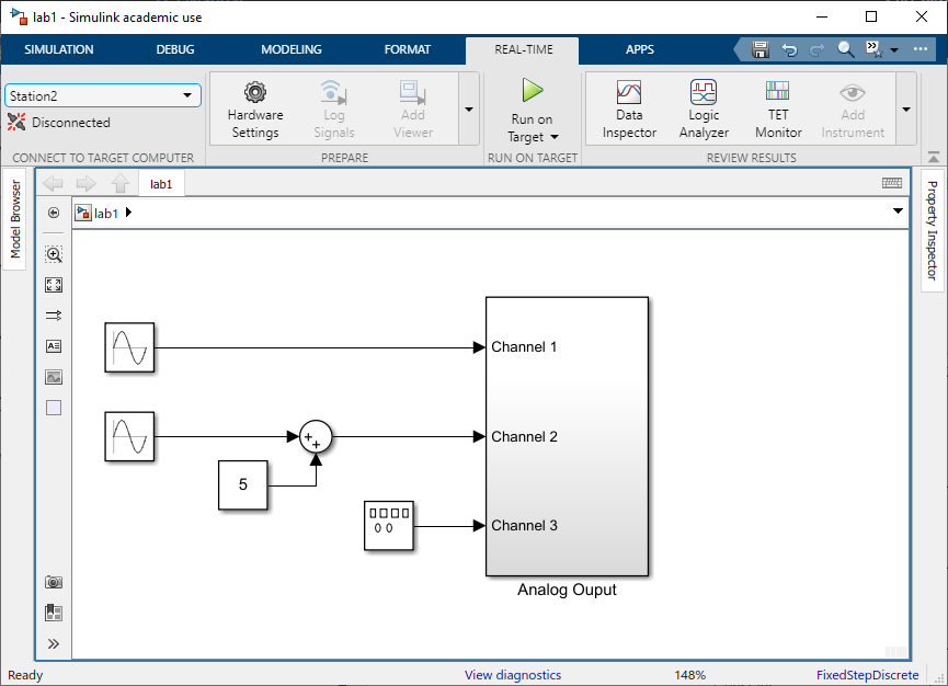

Fig. 1.5 Simulink project window for Lab 1.#

In the model window, double-click on the appropriate source block and use the mouse and keyboard to set up the following 50-Hz waveforms on the D/A outputs:

Note

Some block parameters are in radians.

Table 1.1 Target model parameters#
D/A	Wave Type	Amplitude	DC level	Phase Shift	Oscope	Scale
Ch 1	Sine	\(\qty{5}{\V}\)	\(\qty{0}{\V}\)	\(\qty{0}{\degree}\)	Ch 1	\(\qty{5}{\V\per div}\)
Ch 2	Sine	\(\qty{5}{\V}\)	\(\qty{5}{\V}\)	\(\qty{-90}{\degree}\)	Ch 2	\(\qty{5}{\V\per div}\)
Ch 3	Square	\(\qty{5}{\V}\)	\(\qty{0}{\V}\)	\(\qty{0}{\degree}\)	Ch 3	\(\qty{5}{\V\per div}\)

Simulink Real-Time (slrt) is included in the Simulink software. This software provides the link between the model code and the test hardware. When a model is initially created, default parameters define the simulation environment. Bring to focus the lab1.slx window. Select the Modeling tab. Then press Model Settings button. In the left column of newly created window, select Solver. The window should now appear similar to Fig. 1.6. Change all settings to match Fig. 1.6.

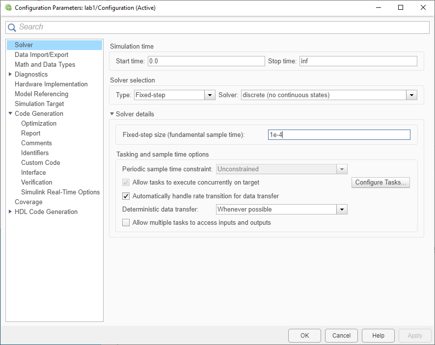
Fig. 1.6 Solver parameters for Lab 1.#

Next, select Code Generation in left column of same window, which should now be similar to Fig. 1.7. Select System target file to match that in Fig. 1.7. Close given window. Bring back to focus the lab1.slx window, which should now have a tab called Real Time. Select this tab. Near top-left corner, select the target PC and press Disconnect link to connect. If everything was successful, the top-left link should now display Connected. If so, press Run on Target button.

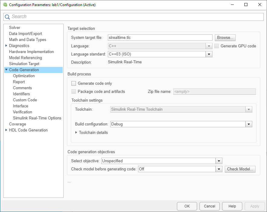
Fig. 1.7 Code generation parameters for Lab 1.#

Simulink will now generate and compile code to run on target PC. This may take a minute or two. If successful, the code will automatically download to and start target model. Confirm by looking at the target display.
Connect amplifier Channels 1, 2 and 3 to oscilloscope Channels 1, 2 and 3, respectively. Trigger on Channel 1. Adjust the time base to capture 2 cycles of data. Display all scope channels.
Apply the D/A Channel 3 voltage to a 25-\(\Omega\) resistor. Measure the current by connecting the lower BNC connector to oscilloscope Channel 4.
To download the oscilloscope data, open BenchVue on the host computer. Exit the demo screen and select the proper oscilloscope. You should see an image of the oscilloscope screen on the host computer. On the screen image tab check the boxes that invert colors (so as not to waste ink or toner when printing), black and white and click get current screen. You should see an image similar to Fig. 1.8. To save your screenshot, select Export in the lower right corner of the BenchVue window. Hit browse, and navigate to your ECE323 folder. Select the lab1 folder and hit OK. This will ensure that BenchVue saves your screenshot in the correct location on your account.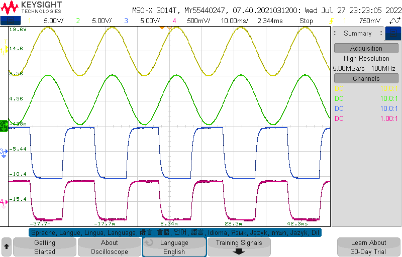

Fig. 1.8 Sample screen shot.#
Next, on the trace data tab, select get current traces. Export the data into MATLAB. When saving the file, make sure the filename you select (e.g. lab1\data) does not include any spaces. Also, uncheck the check-box include number. This will avoid compatibility issues with MATLAB.
Exit or close BenchVue. The waveform data will be stored in a file named lab1\data.mat. The data file contains an \(N \times 2\) matrix of data for each channel of the oscilloscope screen. The first column of each matrix contains the time data. The second column contains the y-axis data of the signal. Some commonly used MATLAB commands are listed at the end of this handout. For more detailed information on using any of these commands, type help command in the MATLAB command window.
Create and execute an m-file containing the following commands that load four channels of oscilloscope data into MATLAB workspace:
```
load lab1_data.mat
time = Trace_1(:,1);
channel1 = Trace_1(:,2);
channel2 = Trace_2(:,2);
channel3 = Trace_3(:,2);
channel4 = Trace_4(:,2);
```
Plot the four channels of data on the computer screen using the MATLAB commands plot and subplot. Add a title, labels, and grid. Make a hard copy printout of the plot.
For each channel, compute the average and RMS values of the signals. This can be accomplished by creating MATLAB programs. Using the m-file editor, write the following MATLAB commands and save in file avg.m.
```
avsum = 0.0;
for i = 1: length(channel1)
    avsum = avsum + channel1(i);
end
av = avsum/length(channel1);
```
When in the MATLAB command window, type avg. The average value of the Channel 1 data will be computed. Repeat this for Channels 2, 3, and 4. Create a MATLAB program to compute the RMS value of each channel. Do NOT use the built-in MATLAB rms command. The RMS value of a continuous signal is defined as

(1.1)#\[\hat x = \sqrt {\frac{1}{T}\int_0^T {{x^2}(t)dt} }.\]

The discrete counterpart is

(1.2)#\[\hat x = \sqrt{\frac{1}{N}\sum_{n = 0}^N {{x^2}(n)} } %\hat x = \sqrt{\frac{1}{N}\sum\nolimits_{n = 0}^N {{x^2}(n)} }\]

where \(N\) is the number of samples in an integer number of periods of the signal. For those who would like to learn more about MATLAB, there are numerous MATLAB reference books available at local bookstores. Also, there is extensive online help - simply type help from the MATLAB command line. Write the results of the calculations on the printouts of the generated plots. Do the results look reasonable?
Staple and turn in all printouts with you name on top of all pages.

1.3. Postlab Exercise: Standalone Simulink model#

In this part, we will develop a standalone computer simulation on the host computer using Simulink. The purpose is to become familiarized with some of the basic building blocks of Simulink, to build a model of a simple dynamic system, learn the steps needed to perform a simulation study and to generate annotated and labelled plots.

Consider the equivalent circuit shown in Fig. 1.9. Using the basic equations of an inductor (\(v=L\frac{di}{dt}\)), and Kirchhoff’s voltage law (KVL), express the dynamic equations of the circuit in the following form

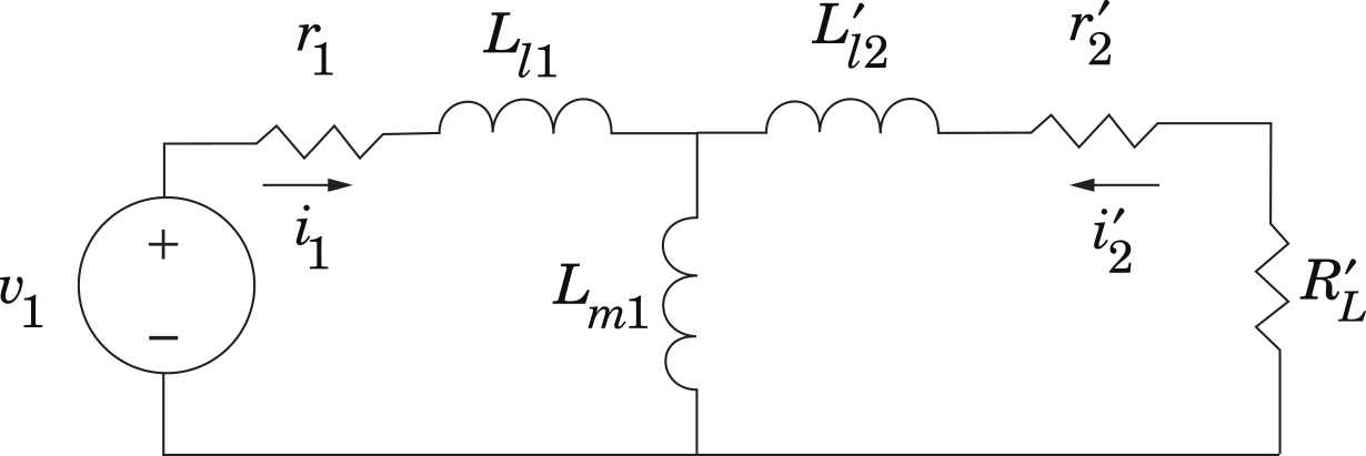
_images/xfmer.png — Fig. 1.9 Example circuit.#

(1.3)#\[\begin{split}\begin{bmatrix} v_1 \\ 0 \\ \end{bmatrix} = \begin{bmatrix} \blank & \blank \\ \blank & \blank \\ \end{bmatrix} \begin{bmatrix} i_1 \\ i_2^\prime \\ \end{bmatrix} + \begin{bmatrix} \blank & \blank \\ \blank & \blank \\ \end{bmatrix} \frac{d}{{dt}} \begin{bmatrix} i_1 \\ i_2^\prime \\ \end{bmatrix}\end{split}\]

where \(i_1\) and \(i_2^\prime\) are the so-called state variables. Replace each of the blanks with expressions involving the circuit parameters. The previous equation may be expressed symbolically as

(1.4)#\[\mathbf{v} = \mathbf{Ri} + \mathbf{L} \frac{d}{dt} \mathbf{i}\]

Equivalently

(1.5)#\[\frac{d}{dt} \mathbf{i} = \mathbf{L}^{-1} ( \mathbf{v} - \mathbf{Ri} )\]

We will build a Simulink model based on this equation. The parameters are given in Table 1.2.

Table 1.2 Model parameters.#
\(r_1\)	\(r_2^\prime\)	\(L_{l1}\)	\(L_{l2}^\prime\)	\(L_{m1}\)	\(R_{L}\)
\(\qty{0.1}{\ohm}\)	\(\qty{0.1}{\ohm}\)	\(\qty{1}{\mH}\)	\(\qty{1}{mH}\)	\(\qty{10}{\mH}\)	\(\qty{1.9}{\ohm}\)

Launch MATLAB, then launch Simulink by pressing the Simulink icon shown in Fig. 1.10. This opens a blank Simulink model window similar to that shown in Fig. 1.10. Note that the default name of the model is untitled. Immediately save this model as mylab1.slx. It is useful to save often since Simulink may occasionally “crash” causing all work since the last save to be lost. Press the Simulink Library icon to open the Simulink Library Browser. From the Simulink Library, open Commonly Used Blocks.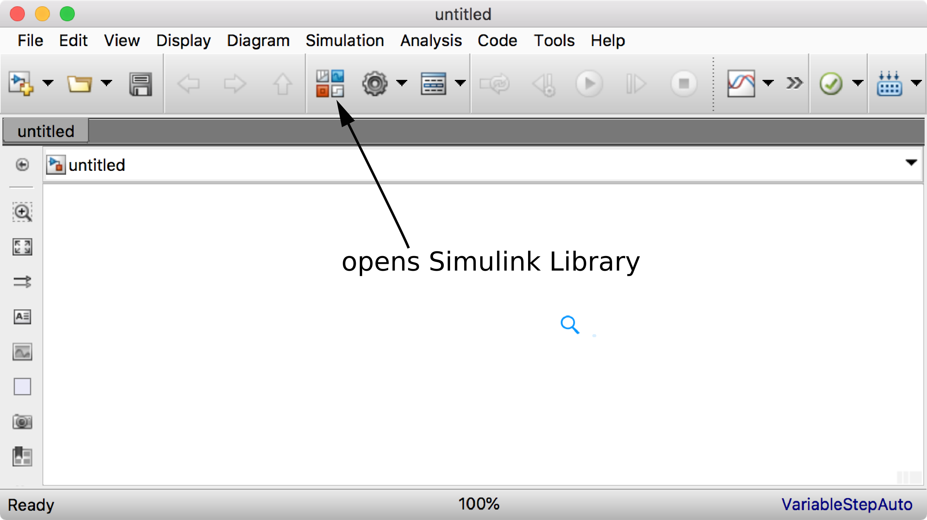

Fig. 1.10 Blank Simulink model window.#
Drag the following blocks from the browser into the empty model window: Sum, Integrator, Gain, Scope, Constant, and Mux. From Simulink/Sinks in the Library Browser, drag the To Workspace block into the model window. From Simulink/Sources, drag the Sine Wave block into the model window.
If the input of the Integrator is set to the right-hand side of (1.5), which is \(d\mathbf{i}/dt\), then the output becomes \(\mathbf{i}\). Note that Simulink uses the Laplace operator \(1/s\) to denote integration with respect to time. This might lead some to believe that Laplace, transform techniques are used to solve the differential equations; however, this is definitely not the case. This is just a symbolic way to say that the output is equal to the input integrated with respect to time. By dragging and connecting the inputs and outputs of the various blocks in accordance with (1.5), form a Simulink model of the given circuit similar to that shown in Figure Fig. 1.11.

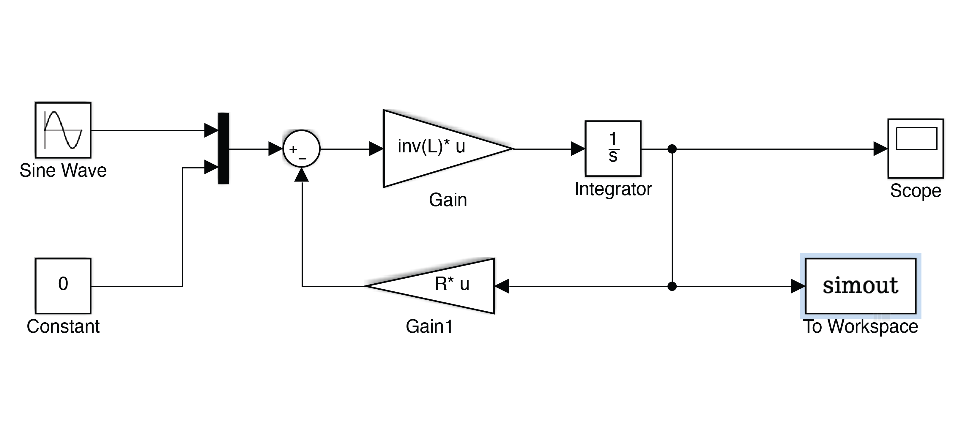
Fig. 1.11 Simulink model.#
In this model, the directed lines (lines with arrows) in the Simulink model represent 2-dimensional signals that connect the output of a block to the input of another block. The two components of the output of the integrator block represent \(i_1\) and \(i_2^\prime\). In accordance with (1.5), the gain in the triangular block preceding the Integrator must be set to \(\mathbf{L}^{-1}\). This is accomplished by double-clicking the Gain block to open its dialog window. In this window, select Matix (K*u) from the pull-down field labelled multiplication and type inv(L) into the text field labeled Gain. You may wish to read more about this block by pressing the help button to open its documentation window. Follow similar steps to set the gain of the other gain block Gain1 to R. We will describe how to define the values of L and R a little later.
The voltage vector \(\textbf{v}\) in (1.5) is a 2-dimensional vector. However, the output of the Sine-Wave block is a scalar signal. To form a 2-dimensional voltage vector, a multiplexer or mux block is used as shown in Fig. 1.11. This block converts the two scalar signals into one 2-dimensional signal. The summer accepts two 2-dimensional inputs and outputs a 2-dimensional signal. If the inputs were of differing dimensions, an error message would be produced when attempting to run the model.
Double-click the Integrator block to open its dialog window. In the dialog window, set the initial condition to [0;0].
To set the parameters for the model, you will create a MATLAB script file named init.m where you will define the values of all parameters. For example,
```
r_1 = 0.1; % primary resistance in Ohms
...
L_l1 = 1e-3; % primary leakage inductance in Henries
...
L = [? ?; ? ?];
R = [? ?; ? ?];
...
```
When you run the script file, the parameters are loaded into the MATLAB workspace. The Simulink model has access to all workspace variables.
Double-click the Sine Wave icon to open its dialog window. Set the amplitude to 100 (volts peak) and frequency to \(\qty{400}{\radian\per\second}\).
Before running the simulation, go to the top menu in the Simulink model window and select the Modelling tab. Then press Model Settings icon. This will open a very important dialog window. Set the solver type to variable step, the maximum step size to 0.1, the minimum step size to 1e-20, and the solver to ode23s. Also, set tstop to 0.5. Step sizes and tstop have units of seconds. Leave the other parameter set to their default values. Double-click the To Workspace block. Make sure the save format is set to Timeseries and sample time to -1.
You are now ready to make a study. Before you do Save! Then press the Run icon. You can double-click the Scope to see if the run is successful.
Although you can print the Scope data from the Scope window, it is preferable instead to generate labelled and annotated printable figures from MATLAB. Create another script file and label it plotresults.m. Enter the following lines
```
figure(1)
plot(simout.time, simout.Data(:,1))
title('i_1')
xlabel('time (sec)')

figure(2)
plot(simout.time, simout.Data(:,2))
title('i_2^\prime')
xlabel('time (sec)')
```
From the two figure windows, use Tools/Data Cursor to determine the peak values of \(I_1(t)\) and \(I_2^\prime (t)\) [steady-state \(i_1(t)\) and \(i_2^\prime(t)\)]. Save the figures as .png files.

1.4. Postlab#

Using phasor analysis, calculate \(\tilde{I}_1\) and \(\tilde{I}_2^\prime\). Express \(I_1(t)\) and \(I_2^\prime(t)\). What are their peak values? Compare the calculated results with the simulated values established in lab.
Submit printouts of the generated plots and all supporting calculations. If you used MATLAB to perform calculations, submit the script file or command history.

1.5. MATLAB Command Reference#

Command	Description
`load file`	Load data stored in `file`
`save array file`	Store a variable array into `file.mat`
`fft(array)`	returns a complex array of fft harmonic components
`^2`, `sqrt()`	square/square root of a variable
`sign`, `abs(array)`	sign/absolute value of a variable/array
`sin`, `cos`, `tan`	sine/cosine/tangent of angle (in radians)
`asin`, `acos`, `atan`	arcsin, arccosine, arctangent
`sinh`, `cosh`, `tanh`	hyperbolic sine, hyperbolic cosine, hyperbolic tangent
`length(array)`	number of elements in an array
`min`, `max`, `mean`	minimum, maximum, and mean of an array
`plot(x,y,x,y..)`	create a screen plot of the arrays y vs x. Also used as `plot(y)`
`title('myplot')`	Add a title to a screen plot
`xlabel('horiz')`	Add an x axis label to a screen plot
`ylabel('vert')`	Add a y axis label to a screen plot
`grid`	Add grid lines to a screen plot
`print`	Dump the screen plot to the printer
`whos`	List current variables and sizes in memory
`clear array`	remove a variable/array from memory
`...`	ellipsis for continuation of long lines
Other Misc.
`! syscommand`	Execute a system command
`dir` or `ls`	list DOS files in current directory
`help ?`	List MATLAB commands and script (.m) files
`quit` or `exit`	end MATLAB program
`linspace(x1,x2,N)`	generates N points between x1 and x2
`hold on`	subsequent plot commands add to existing plot
`subplot`	create a “vector” or “matrix” of plots
`figure`	open a new figure window for plotting