Inductance and Magnetic Circuits

2. Inductance and Magnetic Circuits#

Objective

The main objective of this experiment is to analyze a simple magnetic system with mechanical motion. In particular, a cylindrical electromechanical relay (solenoid) will be analyzed to predict its electromagnetic characteristics. The results of the analysis will be compared with measured results.

2.1. Introduction#

In this experiment, we will investigate the electromagnetic properties of a cylindrical solenoid. A simplified cutaway view of the solenoid is shown in Fig. 2.1. The coil is wound such that an axial magnetic field is produced in the moveable plunger. This magnetic field circulates around the outer shell forming closed flux lines.

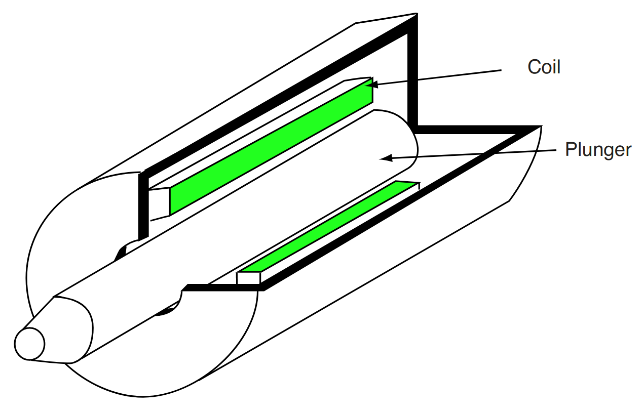
_images/fig1.png — Fig. 2.1 Simplified cutaway view of cylindrical solenoid.#

A cross-sectional view of the solenoid along with representative lines of magnetic flux are shown in Fig. 2.2. The strength of the magnetic field is dependent upon the amount of current in the coil and the displacement of the plunger, $x$. In the prelab, it will be shown that the inductance of the coil (ratio of flux linking the coil to the current flowing in the coil) may be approximated for this solenoid as

(2.1)#\[L(x) = L_l + (K/(k_0 + x))\]

Hopefully, our experimental measurements will confirm the general form of this equation.

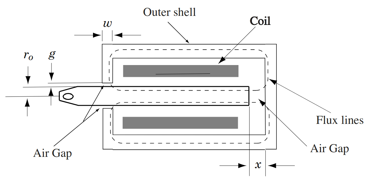
_images/fig2.png — Fig. 2.2 Simplified cross-sectional view of cylindrical solenoid.#

2.2. Prelab#

Before you begin this prelab, it is necessary to be familiar with the material in Sections 1.2 and 1.7 of Electromechanical Motion Devices by Krause and Wasynczuk (hereafter abbreviated as KWP). If you are currently taking EE321, you should read these sections first. It would be beneficial to read Section 1.4 as well.

In this experiment, we will investigate the electrical properties of the solenoid shown in Fig. 2.1Figure 2-1. The coil is wound such that an axial magnetic field is produced in the movable plunger (i.e. along the length of the plunger). This magnetic field crosses the air gap and circulates around the outer shell forming closed flux lines as shown in the sideway cross-sectional view of Fig. 2.2. The magnetic flux density is dependent upon the amount of current in the coil and the displacement of the plunger, $x$. In this prelab, we will establish an expression for the self-inductance of the coil in terms of the displacement, $x$, of the plunger. Using this expression, we will later relate the electromagnetic force to the current $i$ and displacement $x$. This will be done in the next lab.

In the following analysis, we will assume that the magnetic materials (plunger, outer shell, end plates) have infinite permeability (i.e. $\mu_r = \infty$). Otherwise, we would have an analytical mess. Also, we will assume that the lines of magnetic flux in the air gap between the plunger and the end plate on the right-hand side of Fig. 2.1 are uniformly distributed and are constrained to the volume whose cross sectional area is equal to that of the plunger and whose length is $x$.

Using these assumptions, establish and express, in terms of $x$ and $r_0$, the reluctance of the magnetic circuit associated with the air gap between the plunger and right-hand plate}. Specifically, express

(2.2)#\[\mathcal{R}_1 = (\text{some function of $r_0$ and $x$})\]

A second air gap exists in the end plate on the left-hand side of Fig. 2.2. The cross-sectional area of this air gap is $2\pi(r_0+g) w \approx 2\pi r_0 w$ and the length is $g$. Establish and express the reluctance associated with the gap $g$. Specifically,

(2.3)#\[\mathcal{R}_2 = (\text{some function fo $g$, $w$, and $r_0$})\]

Let $N$ represent the total number of turns associated with the coil. The self-inductance may be expressed as

(2.4)#\[L(x) = \frac{N^2}{\mathcal{R}(x)}\]

Relate $K$ and to the geometric variables $g$, $r_0$, and $w$.

(2.5)#\[K = \blank \henry\meter\]

(2.6)#\[k_0 = \blank \meter\]

Using the following parameters, calculate $K$ and $k_0$ (in metric units). Using $K$ and $k_0$ in metric units, plot the inductance versus position from 0 to $\qty{0.0127}{\meter}$ ($\qty{1/2}{\inch}$).

Table 2.1 Solenoid inductance model parameters.#
N	g	$r_0$	w
3740	$\qty{0.0045}{\inch}$	$\qty{0.21}{\inch}$	$\qty{0.48}{\inch}$

Note

$\mu_0 = 4\pi \times 10^{-7} \henry\per\meter$ (Henries/meter). Watch units when calculating inductance.

Let $v$ be the voltage applied to the coil. Express the voltage equation in the form

(2.7)#\[\frac{di}{dt} = (\text{some function of $x$, $i$, $v$, and $\frac{dx}{dt}$})\]

Hint

Apply Product and Chain rules of differentiation to $\displaystyle{v = ri+\frac{d}{dt}[L(x)i]}$.

You should also read through the experiment and postlab sections before coming to the laboratory.

2.3. In the Laboratory#

2.3.1. Inductance versus frequency#

Our first objective in the laboratory will be to measure the inductance of the coil at various frequencies using a sinusoidal applied voltage. To set the position to $x=0$, remove the screw completely. Then hold the plunger against its stop and reinsert the screw turning it until it makes contact with the plunger. Each subsequent turn increases $x$ by $\qty{1/32}{\inch}$. However, we will initially want $x=0$.

Measure coil resistance#

Determine the patch panel voltage and current offset by measuring the current and voltage out of Channel 3 with no voltage applied. Be sure to subtract this offset from your voltage and current values when calculating the resistance.
Create a Simulink model such that Real Time Workshop will provide a DC signal to Channel 3. Apply $\qty{12}{\volt}$ DC to the solenoid coil.
Measure the DC current flowing though the coil. Note: keep current probe away from the magnetic field of the solenoid.
Calculate the coil resistance $R = V/I$.

Measure coil impedance versus frequency#

Create a Simulink model such that Real Time Workshop will provide a sine wave to Channel 3.
Generate a $10$-$\volt$ zero to peak ($\qty{10}{\volt}$ amplitude) $1$-$\hertz$ sine wave. Connect the amplifier output to the solenoid and measure the voltage with the oscilloscope. Make sure the solenoid plunger is completely in (at $x = 0$). Measure the peak-to-peak solenoid current with the oscilloscope.
Repeat the current measurement at higher frequencies ($1$, $2$, $4$, $7$, $10$, $20$, $40$, $70$, and $\qty{100}{\hertz}$). Double check that the frequency inputted into Simulink is in converted to $\radian\per\second$.

Calculate inductance versus frequency#

Calculate the impedance $Z$ at each frequency by taking the ratio of peak-to-peak voltage ($\qty{20}{\volt}$) to the measured peak-to-peak current.
Plot impedance magnitude versus frequency. This may be accomplished with the help of Matlab. A sample set of Matlab instructions is given in Appendix A.
Establish the solenoid’s inductance from the magnitude of impedance at each frequency. Record the largest value for use in the postlab. (Hint: what should the plot look like when $\left | Z \right | = \left | r + j \omega L \right| = \sqrt{r^2 + \omega_e^2 L^2}$ is plotted as a function of $\omega_e$)

2.3.2. Inductance versus position#

Our next objective in the laboratory will be to measure the inductance of the coil at various mechanical displacements.

Measure coil impedance vs position#

Use the sine wave generator Simulink model to provide a sine wave to Channel 3.
Generate a $10$-$\volt$ (zero to peak) $10$-$\hertz$ sine wave using the power amplifier.
Connect the patch panel output to the solenoid and measure peak-to-peak solenoid voltage with the oscilloscope.
Position the solenoid plunger at $x = 0$ (all the way in).
Measure the peak-to-peak solenoid current with the oscilloscope.
Repeat the current measurements by extending the plunger from $0$ to $\qty{1/2}{\inch}$ in $\qty{1/32}{\inch}$ increments ($1$ turn of set screw = $\qty{1/32}{\inch}$).

Calculate inductance versus position#

Calculate the solenoid inductance at each position [Hint: $\left| Z \right| = \sqrt{r^2 + (\omega_e L)^2}$]. This may be accomplished with the help of Matlab. A sample set of Matlab instructions is given in Appendix A.
Plot the inductance versus plunger position.

Calculate $K$ and $k_0$#

Carefully examine the numerical procedure described in Appendix B.

Using the data for inductance versus position obtained above, define x and L_meas in Matlab.
```
x = [...]';
L_meas = [...]';
```
Make sure that x and L_meas are column vectors. Transpose them if they are row vectors.
Define the initial guess vector for $a = \begin{bmatrix} L_l & K & k_0 \end{bmatrix}'$.
```
a = [0.001 0.001 0.0001]'
```
Call the solenoid function $20$ times to iterate to a final value for $\begin{bmatrix} L_l & K & k_0 \end{bmatrix}'$.
```
for i = 1:20
    [a_new, L_fit] = solenoid(L_meas, x, a);
    a = a_new;
end
```
Plot the fitted and measured inductance versus position on a single plot. These plots should agree. If not, repeat with smaller values in the initial guess vector.
Record the final values of $L_l$, $K$, and $k_0$. These are the final converged values in a.

2.4. Postlab#

Plot the measured impedance-versus-frequency characteristics with $x=0$. Superimpose the calculated impedance-versus-frequency characteristics of an ideal circuit using the largest value of inductance from your $\left | Z \right |$ versus $\omega_e$ data. Describe the differences.
The deviations that should be observed in 1., may be attributed to eddy currents induced in the plunger. The presence of eddy currents may be explained with reference to Fig. 2.5. Assume the current in the coil is increasing with respect to time in accordance with the reference direction shown in Fig. 2.5. This will cause the flux to increase in the direction shown (determined by the right-hand rule). The plunger is made of magnetic steel, which is a good conductor. Currents will be induced in the plunger to oppose the increase in flux – this is Lenz’s law. These currents are shown in Fig. 2.5 as dots and crosses but in reality they are continuously distributed inside the plunger. We could calculate these currents using Maxwell’s equations, but this would be a non-trivial task even for an experienced “magneticist”. We will not do this, but we must acknowledge the presence of these currents. Since these eddy currents oppose changes in flux, what effect would they have upon the impedance-versus-frequency characteristics when compared to the case where eddy currents do not exist, which would occur if the plunger were made of a nonconductive material? Explain briefly.

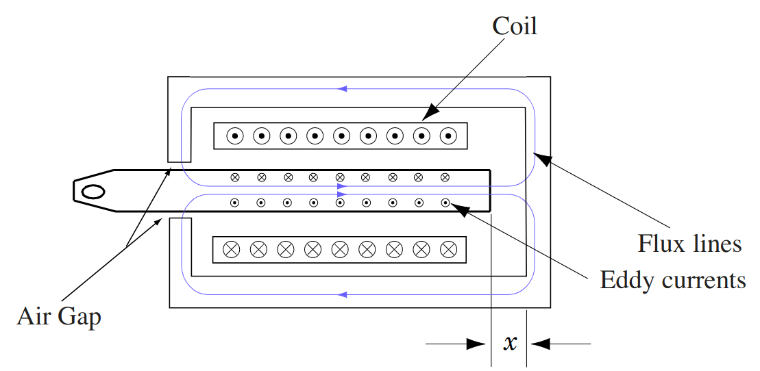
Fig. 2.5 Simplified cross-sectional view of cylindrical solenoid illustrating eddy currents and flux lines.#
For low frequencies, the induced eddy currents will be small because the flux does not change very rapidly. Therefore, they may be ignored. However, if the frequency is too small, it is difficult to extract the inductance from using the formula. Why? Explain briefly.
Based upon the measured impedance-versus-frequency characteristics, for what frequency or range of frequencies would you expect the formula to give an accurate measure of the DC or low-frequency inductance?
Why does the solenoid inductance decrease as the air gap increases?
How does the assumption that the magnetic materials have infinite permeability affect the inductance?
How would saturation affect the inductance?
How could we determine whether magnetic saturation affected our results (e.g. what additional data might we measure)? Hint: saturation is a nonlinear phenomenon. If a sinusoidal voltage is applied to a nonlinear inductor, do you expect the current to be sinusoidal?

2.5. Appendix A: Plotting Measured Data#

% Plotting Impedance versus Frequency. Calculating Inductance
freq = [1,2,4,7,10,20,40,70,100]';
omega_vector = 2*pi*freq;
r = measured resistance;
v1 = [Your Data Points seperated by commas]'; % Volts (Peak-to-Peak)
ipeak1 = [Your Data Points seperated by commas]'; % Amperes (Peak-to-Peak)
z1 = v1./ipeak1;
L_vs_f = sqrt(z1.^2 - r^2)./omega_vector;
figure(1)
plot(freq,z1,'*')

% Plotting Inductance versus Position
omega_constant = 2*pi*10;
x = [0,1,2,3,4,5,6,7,,8,9,10,11,12,13,14,15,16]';
x = x/32; % Convert to Inches
x = x/39.37; % Convert to Meters
v2 = 20; % Volts (Peak-to-peak)
ipeak2 = [Your Data Points seperated by commas]'; % Amperes (Peak-to-Peak)
z2 = v2./ipeak2;
L_vs_pos = sqrt(z2.^2 - r^2)/omega_constant;
figure(2)
plot(x, L_vs_pos,'*');

2.6. Appendix B: Establishing Analytical Approximation of Measured Data#

It is desired to approximate the inductance in the form

(2.8)#\[L(x) = L_l + \frac{K}{k_0 + x}\]

where $L_l$ represents stray or leakage inductance. Equivalently,

(2.9)#\[L(x) = a_1 + \frac{a_2}{a_3 + x}\]

Define $e_i$ as the difference between the calculated and measured inductances at $x_i$

(2.10)#\[e_i = a_1 + \frac{a_2}{a_3 + x} - L_i\]

Define $E$ as

(2.11)#\[E = \sum\limits_{i = 1}^N (e_i)^2 = \sum\limits_{i = 1}^N (a_1 + \frac{a_2}{a_3 + x_i} - L_i)^2 \]

where $N$ is the total number of measured data points. The values of $a_1$, $a_2$, and $a_3$ that minimize $E$, satisfy the following equations

(2.12)#\[0 = \frac{\partial E}{\partial a_1} = \sum\limits_{i = 1}^N 2\left( a_1 + \frac{a_2}{a_3 + x_i} - L_i \right) = f_1(a_1,a_2,a_3)\]

(2.13)#\[0 = \frac{\partial E}{\partial a_2} = \sum\limits_{i = 1}^N 2\left( a_1 + \frac{a_2}{a_3 + x_i} - L_i \right) \frac{1}{a_3 + x_i} = f_2(a_1,a_2,a_3)\]

(2.14)#\[0 = \frac{\partial E}{\partial a_3} = \sum\limits_{i = 1}^N 2\left( a_1 + \frac{a_2}{a_3 + x_i} - L_i \right) \frac{1}{(a_3 + x_i)^2} = f_3(a_1,a_2,a_3)\]

Symbolically,

(2.15)#\[\bs{0} = \bs{f}(\bs{a})\]

Taylor series gives

(2.16)#\[\bs{0} = \bs{f}(\bs{a}_\text{guess}) + \left. \frac{\partial \bs{f}}{\partial \bs{a}} \right|_{\bs{a}_\text{guess}} \left( \bs{a} - \bs{a}_\text{guess} \right) + \cdots \]

Rearranging

(2.17)#\[\bs{a} \approx \bs{a}_\text{guess} + \left. \frac{\partial \bs{f}}{\partial \bs{a}} \right|_{\bs{a}_\text{guess}}^{-1}\bs{f} (\bs{a}_\text{guess}) =\bf a_\text{new}\]

The previous equation defines an iterative method of estimating $\textbf{a}$, given an initial guess, $\textbf{a}_{\rm guess}$. A printout of a Matlab function which calculates given is attached. This function is stored in the file solenoid.m. This function may be called repeatedly (each time replacing $\textbf{a}_{\rm guess}$ with $\textbf{a}_{\rm new}$) until $\textbf{a}_{\rm new}$ converges to ${\bf a}$.

function [a_new, L_fitted] = solenoid(L_meas,x,a);
    % L_meas = n vector of measured inductances
    % x = n vector of displacements
    % a = Initial guess vector of fitted parameters
    % a_new = Better guess vector of fitted parameters
    % L_fitted(i) = n vector of fitted inductances
    
    N = length(L_meas);

    % Calculate residual and Jacobian
    F = zeros(3,1); % 3*1 vector
    J = zeros(3,3); % 3*3 vector
    L_fitted = zeros(N,1);
    for i = 1:N
        F(1) = F(1) + (-L_meas(i) + a(1) + a(2)/ (a(3) + x(i)));
        F(2) = F(2) + (-L_meas(i) + a(1) + a(2)/ (a(3) + x(i)))/(a(3)+x(i));
        F(3) = F(3) + (-L_meas(i) + a(1) + a(2)/ (a(3) + x(i)))/(a(3)+x(i))^2;

        J(1,1) = N;
        J(1,2) = J(1,2) + 1.0/(a(3)+x(i));
        J(1,3) = J(1,3) - a(2)/(a(3)+x(i))^2;

        J(2,1) = J(2,1) + 1.0/(a(3)+x(i));
        J(2,2) = J(2,2) + 1.0/(a(3)+x(i))^2;
        J(2,3) = J(2,3) - a(2)/(a(3)+x(i))^3;

        J(3,1) = J(3,1) + 1.0/(a(3)+x(i))^2;
        J(3,2) = J(3,2) + 1.0/(a(3)+x(i))^3;
        J(3,3) = J(3,3) - a(2)/(a(3)+x(i))^4;        
    end 

    % Update
    a_new = a - inv(J)*F;

    % Calculate fitted inductance
    for i = 1:n
        L_fitted(i) = a_new(1) + a_new(2) / (a_new(3) + x(i));
    end
return