12. Brushless DC Motor (B)#
Objective
In this experiment, the rotor position of the permanent-magnet synchronous machine considered in Experiment 11 will be measured and used to control the frequency of a variable-frequency source (inverter). The purpose of this experiment is to show that the torque-versus-speed characteristics of the motor-inverter combination, which constitute a brushless DC motor, is similar to that of the conventional permanent-magnet AC machine.
12.1. Introduction#
Using the parameters established in previous experiments, we should be able to predict the torque-versus-speed characteristics of the given brushless DC motor. These characteristics were plotted as part of last week’s postlab. In this lab, we will attempt to verify these characteristics by experimental measurement.
There are several challenges in measuring the torque-versus-speed characteristics of this motor. First, because the motor is relatively small, the friction and windage torques may be sizable relative to the electromagnetic torque. Thus, the reading from the torque transducer, which represents the shaft torque (electromagnetic torque minus the friction and windage torques), may not be an accurate indication of the actual electromagnetic torque except at low speeds where friction and windage effects are less important. In addition, during normal operation, we are not applying sinusoidal voltages (we are applying square-wave voltages). Consequently, the electromagnetic torque will not be constant in the steady state but will vary as a function of \(\theta_r\). Nonetheless, the average torque at a given speed should be in reasonable agreement with the value established using the analytical torque-versus-speed characteristics. The trouble is that we need a means of establishing the average electromagnetic torque (not the average shaft torque).
The measurement of the average torque-versus-speed characteristic will be accomplished in two steps. First, we will measure the so-called static torque-versus-position characteristics. In particular, we will measure the electromagnetic torque as a function of rotor position at stall (\(\omega_r = 0\)). In an ideal brushless DC machine, the electromagnetic torque will be constant (independent of rotor position). However, because of previously mentioned factors, the electromagnetic torque will vary as a function of rotor position. If the torque versus position is averaged over one period (a quarter rotation in an 8-pole motor), the average torque should be reasonably close to the value predicted using the analytical torque-versus-speed formula with \(\omega_r = 0\). Using previously measured data, we should be able to relate the stator currents \(i_{as}\), \(i_{bs}\), and \(i_{cs}\) to the electromagnetic torque. We will verify this relationship for the static case (\(\omega_r = 0\)) and use it for the general case (\(\omega_r \ne 0\)).
Although the following relationships were given in previous lab documents, we will repeat them here for convenience:
where \(\displaystyle \frac{d\lambda_{asm}}{d\theta_r}\), \(\displaystyle \frac{d\lambda_{bsm}}{d\theta_r}\), and \(\displaystyle \frac{d\lambda_{csm}}{d\theta_r}\) are functions of \(\theta_r\). In particular,
12.2. Prelab#
Read the preceding introduction.
12.3. In the Laboratory#
12.3.1. Static Torque-Versus-Position Characteristics#
Connect phase \(a\) to the amplifier output of Channel 1 and phase \(b\) to ground. Leave phase \(c\) unconnected. The output of the position transducer should be connected to the Digital Data Inputs port.
Connect the amplifier output of the torque transducer to Analog Input 1. Set the range of the Channel 1 input to \(\qty{+1}{\V}\) (middle position). Tare the torque transducer before applying voltage to the motor.
The torque-versus-position will be measured using the prebuilt Simulink models
T_vs_pos_tgt.slxandT_vs_pos_host.slx. The top-level views of these models are shown in Fig. 12.1 and Fig. 12.2, respectively.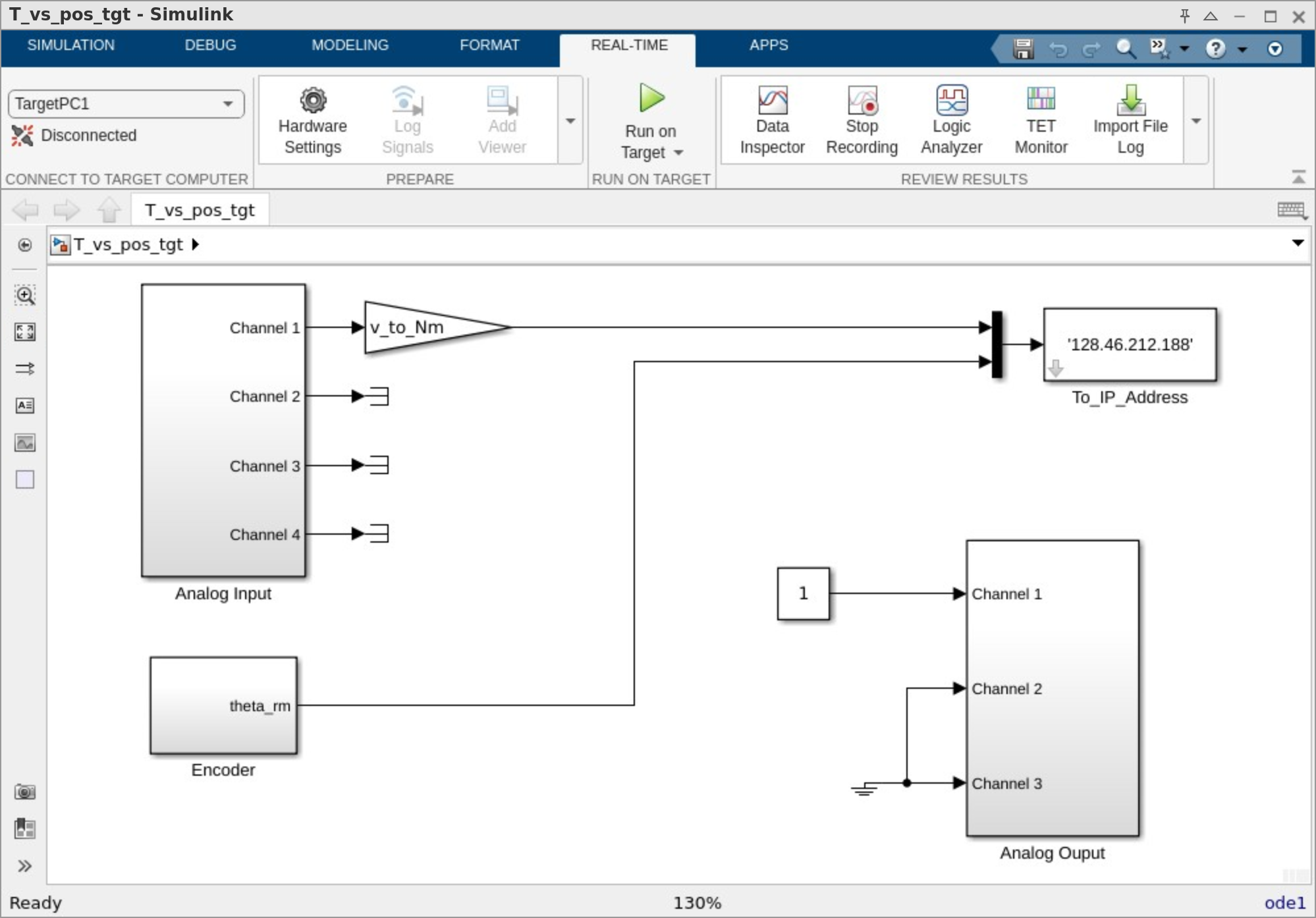
Fig. 12.1 Simulink target model
T_vs_pos_tgt.slxfor measuring torque versus position.#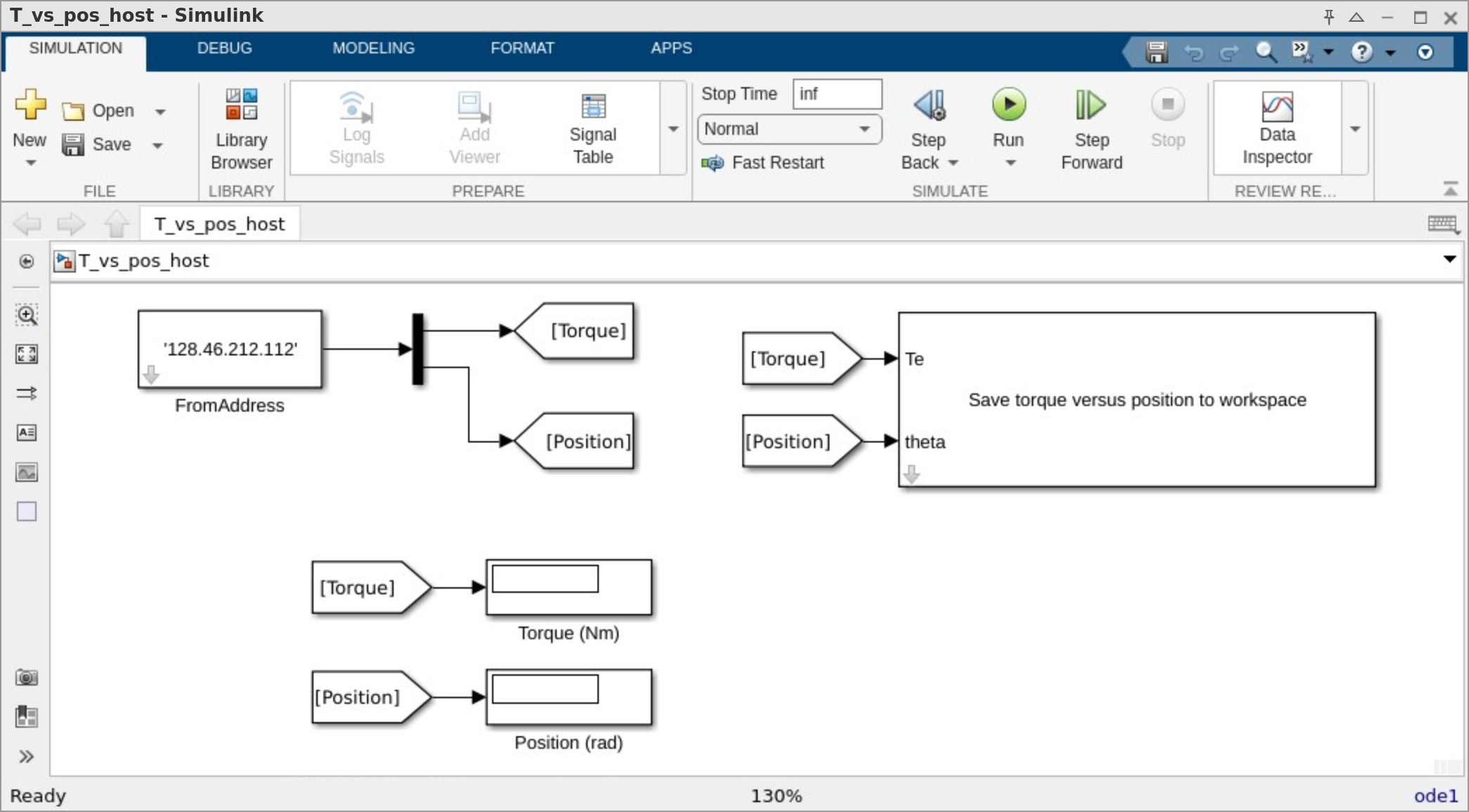
Fig. 12.2 Simulink host model
T_vs_pos_host.slxfor measuring torque versus position.#Open
T_vs_pos_tgt.slx. The model consists of a Constant source, set to 1, connected to Channel 1 of the Analog Output Module, a Ground source connected to the remaining channels of the Analog Output Module, and an Encoder block connected to a Terminator sink. It also includes an Analog Input Module with all ports connected to terminators. Build the model, and confirm a successful build in the View Diagnostics window.The simulation that will run on the host computer is configured as a Normal simulation. This simulation samples the output of blocks in the target computer simulation,
T_vs_pos_tgt.slx. The position and torque of the BDC motor are displayed in digital displays in the model window.Apply a \(\qty{1}{\V}\) DC signal to the phase-\(a\) winding by running the model. Open
T_vs_pos_host.slxand select Run to begin the host simulation. Allow the rotor to settle out to its equilibrium position. Record the position of the rotor from the numeric display. Measure and record \(i_{as} = -i_{bs}\).Using your hand, rotate the motor rotor slowly and smoothly from the encoder end of the torque transducer. As the rotor rotates, the computer calculates a new value of torque for each position the motor rotates through and updates the digital displays of the host simulation.
Use the following MATLAB command line to save the data:
bdctorq ('ta.mat', position, torque)
The resulting data file
ta.matcan be used for subsequent plotting and analysis using MATLAB.Disconnect the power amplifier output from phase \(a\) and connect it to phase \(b\). Connect phase \(c\) to ground. Restart the host simulation and tare the torque transducer. Measure the currents and torque versus position of the phase \(b\) winding as done with the \(a\) winding. Again, save the data in file
tb.mat. Repeat the previous steps for the phase-\(c\) winding with phase \(a\) connected to ground and phase \(b\) disconnected, saving the data intc.mat. Loadta.matinto Matlab. The data will be stored as 2-column matrices of position (\(\radian\)) and torque (\(\newtonmeter\)). Separate the data into vectors of torque and position.qrma = position torquea = torque
Repeat these MATLAB commands for phases \(b\) and \(c\), by loading
tb.matandtc.mat, substituting the appropriate letter for theainqrmaandtorquea. Plot and print the three torque curves.plot(qrma, torquea, qrmb, torqueb, qrmc, torquec)
Print the results and save your Matlab workspace by typing
save lab12_te
Email the file
lab12_te.matto your partner in a zipped folder. You will need this file to complete the postlab. Based upon the measured torque-versus-position characteristic and the measured currents, calculate \(\lambda_m^\prime\). Use the average current to find \(\lambda_{m,ab}^\prime\), \(\lambda_{m,bc}^\prime\), and \(\lambda_{m,ca}^\prime\). Then average to find \(\lambda_m^\prime\). Compare with previously calculated values. Stop simulations.Next, connect phases \(a\), \(b\), and \(c\) to the outputs of Channels 1, 2, and 3, respectively and execute
lab_11_bdc3_target.slxwhich implements the switching algorithm used in last week’s experiment. Turn the motor on, and apply a load torque to the motor to stall the motor. Measure the torque transducer amplifier output voltage on the oscilloscope to establish the shaft torque. Rotate the rotor slowly to determine the maximum shaft torque and record this as the measured stall torque. Tare the torque transducer prior to this test to obtain the correct value.Ask your instructor to disconnect the rotor from the torque transducer (to reduce friction and windage losses) and turn the motor back on. Measure the frequency of the applied voltages \(v_{ag}\), \(v_{bg}\), and \(v_{cg}\) and calculate the no-load electrical speed from the average frequency. Plot the torque-versus-electrical speed characteristic assuming it is a straight line, with the predicted characteristic (from (11.26)) on one axis.
12.4. Postlab#
Plot the predicted torque-versus-electrical speed characteristics and the measured results on the same axis.
Compare analytical and measured stall torques.
Compare analytical and measured no-load electrical speeds.
In each of the above items, provide plausible explanations for any discrepancies between measured and predicted values.