\[ \begin{align}\begin{aligned}\newcommand\blank{~\underline{\hspace{1.2cm}}~} \newcommand\phase[1]{\enclose{phasorangle}{#1}} \newcommand\RE{\mathrm{Re}} \newcommand\IM{\mathrm{Im}}\\% Bold symbols (vectors) \newcommand\bs[1]{\mathbf{#1}}\\% Poor man's siunitx \newcommand\unit[1]{\mathrm{#1}} \newcommand\num[1]{#1} \newcommand\qty[2]{#1~\unit{#2}}\\\newcommand\per{/} \newcommand\squared{{}^2} % % Scale \newcommand\milli{\unit{m}} \newcommand\kilo{\unit{k}} \newcommand\mega{\unit{M}} % % Angle \newcommand\radian{\unit{rad}} \newcommand\degree{\unit{\kern{-0.5ex}{}^\circ}} % % Time \newcommand\second{\unit{s}} % % Distance \newcommand\meter{\unit{m}} \newcommand\m{\meter} \newcommand\inch{\unit{in}} % % Mass \newcommand\gram{\unit{g}} \newcommand\g{\gram} % % Frequency \newcommand\hertz{\unit{Hz}} \newcommand\rpm{\unit{rpm}} % % Voltage \newcommand\volt{\unit{V}} \newcommand\V{\volt} \newcommand\millivolt{\milli\volt} \newcommand\mV{\milli\volt} \newcommand\kilovolt{\kilo\volt} \newcommand\kV{\kilo\volt} % % Current \newcommand\ampere{\unit{A}} \newcommand\A{\ampere} \newcommand\milliampereA{\milli\ampere} \newcommand\mA{\milli\ampere} \newcommand\kiloampereA{\kilo\ampere} \newcommand\kA{\kilo\ampere} % % Resistance \newcommand\ohm{\Omega} \newcommand\milliohm{\milli\ohm} \newcommand\kiloohm{\kilo\ohm} % correct SI spelling \newcommand\kilohm{\kilo\ohm} % "American" spelling used in siunitx \newcommand\megaohm{\mega\ohm} % correct SI spelling \newcommand\megohm{\mega\ohm} % "American" spelling used in siunitx % % Inductance \newcommand\henry{\unit{H}} \newcommand\H{\henry} \newcommand\millihenry{\milli\henry} \newcommand\mH{\milli\henry} % % Power \newcommand\watt{\unit{W}} \newcommand\W{\watt} \newcommand\milliwatt{\milli\watt} \newcommand\mW{\milli\watt} \newcommand\kilowatt{\kilo\watt} \newcommand\kW{\kilo\watt} % % Torque \newcommand\ozin{\unit{oz}\text{-}\unit{in}} \newcommand\newtonmeter{\unit{N\text{-}m}}\end{aligned}\end{align} \]

7. DC Motor (A)

Objective

In this experiment, the steady-state and dynamic characteristics of a permanent-magnet DC motor are investigated. In the first lab session, the fundamental parameters of a DC motor will be measured and the concepts of power transfer and conservation of energy will be demonstrated. In the second session, computer simulation will be used to predict the steady-state and dynamic operating characteristics. The analytical and simulated results will be compared with experimental measurements.

7.1. Prelab

The electromechanical equations of a permanent-magnet DC machine can be expressed

(7.1)\[T_e - T_L = J \frac{d\omega_r}{dt} + B_m \omega_r\]

(7.2)\[v_a = r_a i_a +L_{AA} \frac{di_a}{dt} + k_v \omega_r\]

where

(7.3)\[T_e = k_T i_a.\]

Here, \(T_L\) is the applied load torque and \(v_a\) is the applied armature voltage. If all variables are expressed in SI units, \(k_T = k_v\).

The power delivered to the mechanical load may be expressed

(7.4)\[P_m = T_L \omega_r\]

The electric power delivered to the mechanical load may be expressed

(7.5)\[P_e = v_a i_a\]

During steady-state operation with a constant applied armature voltage and constant load torque, all electrical and mechanical variables will be constant. Express (7.1) through (7.3) assuming steady-state operating conditions. Use upper-case letters to designate steady-state variables.

Assume \(L_{AA}\) is small enough so that it can be neglected. Simplify (7.1)–(7.3) and express the first-order transfer function relating speed \(\omega_r\) to armature voltage \(v_a\) when \(T_L=0\), and \(\omega_r\) to load torque \(T_L\) when \(v_a=0\). Express \(\omega_r(t)\) for a step change in armature voltage from 0 to \(V_a\). You may use either Laplace transform techniques or you can solve the first-order differential equation using the method of undetermined coefficients. Hint: for a first-order transfer function

(7.6)\[\omega_r(t) = \omega_{r,ss} (1-e^{-t/\tau_m})\]

Relate \(\omega_{r,ss}\) and \(\tau_m\) to the machine parameters and \(V_a\). Finally, read through the laboratory procedure before coming to lab.

7.2. In the Laboratory:

Attention

Safety glasses must be worn at all times during this lab.

The rotors of two identical motors (numbered 1 and 2) are connected to the torque transducer as shown in Fig. 7.1.

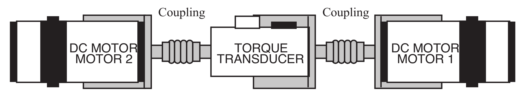
Fig. 7.1 Configuration for measuring voltage constant.

Our first objective will be to measure the electrical parameters \(L_{AA}\) , \(r_a\), and \(k_v\).\

7.2.1. Armature Resistance and Inductance:

1. Block the rotor by hand to prevent it from turning. Using Simulink as in previous experiments, apply \(\qty{2}{\V}\) (DC) to the motor terminals of motor 1 (positive to red, negative to black) through a high-power output channel, \(V_a = \qty{2}{\V}\). Measure the DC current and voltage over motor 1 using the current probe and oscilloscope. Vary the rotor position by hand to determine if the DC current (consequently resistance) varies as a function of the rotor position. Record the maximum, minimum, and average current, then calculate a maximum, minimum, and average resistance \(r_a\) from those currents.

2. Using the Simulink model shown in Fig. 7.2, apply a sinusoidal voltage to the armature terminals

   (7.7)\[V_a=4\sin(200\pi t)\]

   Measure the peak-to-peak current and peak-to-peak voltage. Vary the rotor position by hand and re-measure to see if and by how much \(\left|I_a\right|\) (consequently, the inductance) varies with rotor position. Record the maximum and minimum current magnitude and calculate \(\left| Z \right| = \left| V_a \right| / \left| I_a \right|\) using the average \( \left| I_a \right|\). From \(\left| Z \right|\) and \(r_a\), estimate the motor inductance \(L_{AA}\).

   Hint

   \(\left| Z \right| = \sqrt{r_a^2 + (\omega_e L_{AA})^2}\) .

   

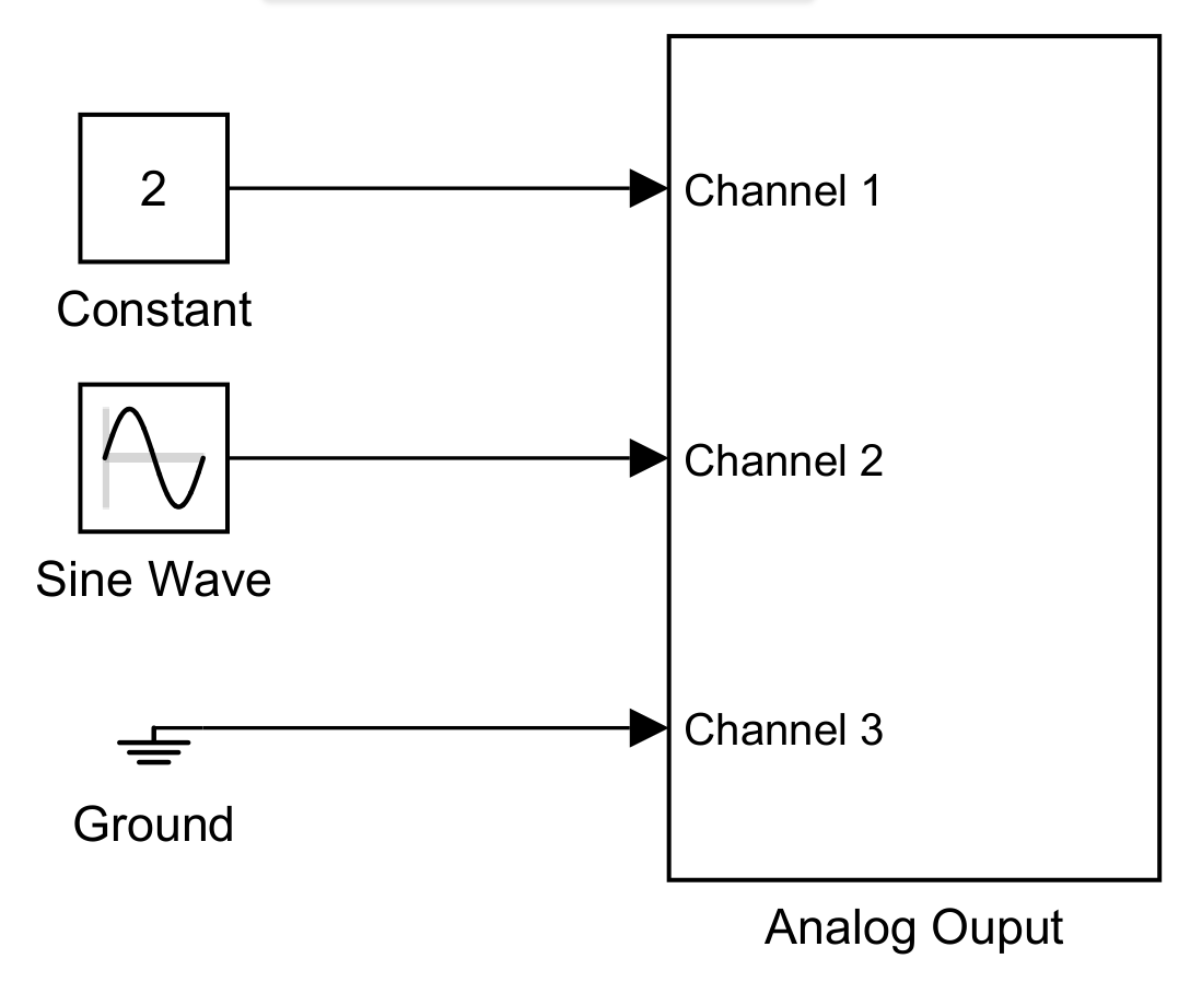
   Fig. 7.2 Simulink target model for DC Motor (A).

7.2.2. Torque constant:

1. Prevent the shaft from turning by holding it between the transducer and motor 2 (see Fig. 7.1). While the rotor is stationary, remove the torque measurement offset by pressing the Tare button on the torque transducer amplifier on your bench.

2. Use the Simulink target model to apply \(\qty{4}{\V}\) (DC) to the armature terminals. Measure the armature current with the lower BNC connector on the same Analog Output module and the torque using the torque transducer amplifier. Connect the current output signal to oscilloscope Channel 1, and the output of the torque transducer amplifier to oscilloscope Channel 2. The output of the torque transducer amplifier is calibrated to produce \(\qty{1}{\V}\) for \(\qty{20}{\ozin}\) of torque. You will later need to convert to SI units.

   Hint

   \(\qty{1}{\newtonmeter} = \qty{141.6}{\ozin}\)

3. Vary the armature voltage of Motor 1 from \(\qty{+4}{\V}\) to \(\qty{-4}{\V}\) in \(1\)-\(\V\) steps, keeping the rotor blocked and recording the armature current and torque transducer output voltage at each step.

4. Calculate and plot the torque (in \(\newtonmeter\)) versus current. Calculate \(k_T\) by creating a line of best fit from the resulting plot, and recording the slope. Express your answer in \({\newtonmeter\per\ampere}\).

7.2.3. Voltage constant:

1. Using the Simulink model, apply \(\qty{8}{\V}\) (DC) to the armature of Motor 2 (causing both motors to rotate). Leave the armature of Motor 1 (test motor) open-circuited.

2. Measure the armature voltage of Motor 1 (its armature is still open circuited) on Channel 1 of the oscilloscope, and the tachometer voltage of Motor 1 on Channel 2 (see Fig. 7.3). Connect the torque transducer amplifier output to Channel 3 of the oscilloscope. This represents a measure of the frictional torque of Motor 1.

   

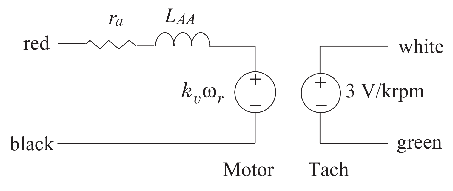
   Fig. 7.3 Equivalent circuit of DC motor/tach.

3. Vary the voltage applied to the armature of Motor 2 from \(\qty{+8}{\V}\) to \(\qty{-8}{\V}\) in \(2\)-\(\V\) steps and record the Motor-1 open-circuit voltage, the tachometer voltage, and the torque transducer output voltage at each step.

4. Calculate the rotor speed from the tach voltage and convert to \(\radian\per\second\). Speed is calculated using \(\omega_r = V_{a,{\rm tach}}/k_{v,{\rm tach}}\) where \(V_{a,{\rm tach}}\) is the tachometer voltage and \(k_{v,{\rm tach}}\) is the tachometer voltage constant (\(\qty{3}{\V\per\kilo\rpm}\)). You should convert the tachometer voltage constant to \(\V\per\radian\per\second\). Plot the open-circuit voltage of Motor 1 versus rotor speed (\(\radian\per\second\)). Generate a best fit line, and determine \(k_v\) from the slope of the given plot. Express the result in \(\V\text{-}\second\per\radian\). Verify that \(k_T = k_v\) when both are expressed in SI units.

   Hint

   \(\qty{1}{\V\text{-}\second\per\radian} = \qty{1}{\newtonmeter\per\ampere}\)

5. From the torque transducer voltage, calculate the frictional torque in \(\newtonmeter\). Plot the frictional torque versus speed. Generate a best fit line, and determine \(B_m\) in \(\newtonmeter\text{-}\second\per\radian\) from the slope of given plot.

7.3. Postlab

1. How much do \(r_a\) and \(L_{AA}\) vary? Why do they vary?

2. What were your experimental values for \(k_T\), \(k_v\), \(r_a\), \(L_{AA}\) and \(B_m\)?

3. What is the relationship between open-circuit voltage and speed? What is the relationship between torque and current? How does this relationship change with rotor speed?

4. What is the relationship between \(k_T\) and \(k_v\)? What was the percentage difference between \(k_T\) and \(k_v\)? Provide possible explanations for this difference.

5. Using the \(r_a\), \(k_v\), and \(k_T\) established in lab, calculate and plot the predicted first quadrant \(T_e\)-versus-\(\omega_r\) characteristics for this motor with \(V_a = \qty{4}{\V}\) (DC). Identify the stall torque (\(T_e\) with \(\omega_r=0\)) and no-load speed (\(\omega_r\) with \(T_e = 0\)).