3. Electromagnetic Forces (A)#
Objective
The primary objective of this experiment is to study the interaction between electrical and mechanical systems that are magnetically coupled. The electromechanical relay (solenoid) studied in Experiment 2 will be analyzed to predict its steady-state force-versus-position and force-versus-current characteristics. In the follow-up lab, computer simulation will be used to predict its dynamic force-versus-time characteristics. The analytical and simulated results will be compared with laboratory measurements.
3.1. Introduction#
In this lab, we will consider the cylindrical solenoid depicted in Fig. 3.1. In the previous experiment, it was shown that the self-inductance can be approximated as
Here, \(K\) and \(k_0\) are assumed to be known constants and \(L_l\) is the leakage inductance. In the prelab, we will establish an expression for the force versus position and set forth the electrical and mechanical equations in state-space form. Hopefully, our experimental measurements will confirm the general form of this equation.
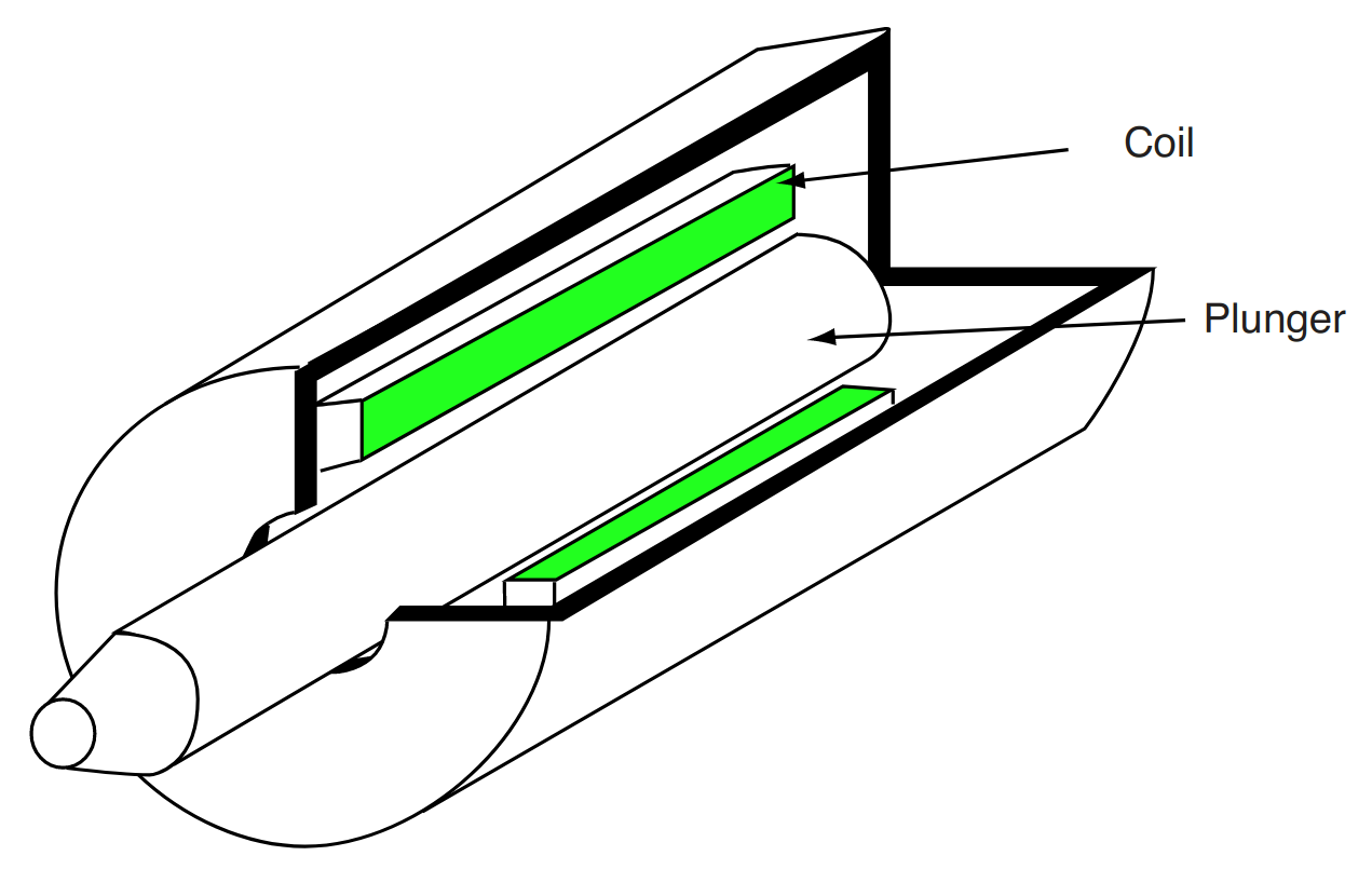
Fig. 3.1 Simplified cutaway view of cylindrical solenoid.#
3.2. Prelab#
For an electromechanical device whose inductance versus position is given by (3.1), express the electromagnetic force as a function of current and position.
(3.2)#\[f_e(i,x) = (\text{some function of $i$, $x$, $K$, $k_0$})\]Using the \(K\) and \(k_0\) values (in metric units) determined in Experiment 2, plot \(f_e\) versus \(i\) for \(0 < i < \qty{200}{\mA}\) and \(x = \qty{0.0032}{\m}\). Plot \(f_e\) versus \(x\) for \(0 < x < \qty{0.0127}{\m}\) and \(i = \qty{200}{\mA}\).
3.3. In the Laboratory#
Attention
You must wear eye protection for this lab.
3.3.1. Force versus Position#
Our first objective will be to measure the force-versus-position characteristics with a constant current. You will need to measure current in the solenoid. A voltage signal proportional to the current is available on one of the BNC connectors of the power amplifier.
Energize the solenoid coil with \(\qty{12}{\V}\) (DC). Use \(R\) from previous experiment, calculate expected current. Measure coil current and compare with expected value. Provide reasonable explanation for any difference. Connect the lower BNC output to the oscilloscope to read the current on an open circuit. Record this value, which will be subtracted from future DC current measurements.
Position the solenoid plunger at \(x = 0\) (the set screw should be all the way out). Add weights to the solenoid plunger until plunger pulls out. Record the mass that is required to just pull the solenoid plunger out to nearest \(\qty{10}{\g}\). Either round up or down but be consistent from one measurement to next.
Caution
Be careful not to drop the weights on your (or your lab partner’s) foot. You may use the lab chairs to prevent dropping weights on the floor.
Repeat the measurements with plunger position varied from \(0\) to \(\qty{1/2}{\inch}\) at \(\qty{1/32}{\inch}\) intervals (1 screw turn = \(\qty{1/32}{\inch}\)). Ensure that the screw is touching the plunger before counting turns. If the minimum (\(\qty{50}{\g}\)) level is reached, then stop.
Calculate the plunger force using \(F=mg\) where \(g = \qty{9.8}{\meter\per\second\squared}\) and \(m\) is the external mass. This is approximately equal to the magnitude of the electromagnetic force developed by the solenoid.
3.3.2. Force versus Current#
Our next objective will be to measure force versus current at a fixed position.
Apply a DC voltage to the coil so that \(i=\qty{60}{\mA}\). Use Ohm’s law to determine the required voltage using the value of \(R\). Measure the current using the oscilloscope to be sure. If necessary, adjust the applied voltage to achieve the desired current. Position plunger at \(x = \qty{1/8}{\inch}\). Add weight to coil plunger until plunger pulls out. Again, be careful not to drop the weights.
Repeat measurements at the same position for coil currents from \(60\) to \(\qty{105}{\mA}\) in \(5\)-\(\mA\) intervals. Record the maximum weight values as the current varies.
3.4. Postlab#
Plot, on the same axis, the measured and calculated electromagnetic force versus current with \(x = \qty{1/8}{\inch}.\) Compare the results and explain discrepancies.
Hint
The most common problem involves mixing Standard International (SI) and English units. It is best to convert all measured data to SI units before making any comparisons.
Plot, on the same axis, the measured and calculated electromagnetic force-versus-position characteristics with constant \(i\). Compare the results and explain discrepancies.