Variable Reluctance Stepper Motor (A)

5. Variable Reluctance Stepper Motor (A)#

Objective

In this experiment, the electromechanical characteristics of a variable-reluctance stepper motor will be investigated. The basic parameters will be measured experimentally and used to predict the static torque-versus-position characteristics.

5.1. Introduction#

The voltage equations of a three-stack variable-reluctance stepper motor may be expressed

(5.1)#\[v_{as} = r_s i_{as} + \frac{d\lambda_{as}}{dt}\]

(5.2)#\[v_{bs} = r_s i_{bs} + \frac{d\lambda_{bs}}{dt}\]

(5.3)#\[v_{cs} = r_s i_{cs} + \frac{d\lambda_{cs}}{dt}\]

where

(5.4)#\[\begin{split}\left[ \begin{array}{c} \lambda_{as} \\ \lambda_{bs} \\ \lambda_{cs} \end{array} \right] = \left[ \begin{array}{ccc} L_{asas} & 0 & 0 \\ 0 & L_{bsbs} & 0 \\ 0 & 0 & L_{cscs} \end{array} \right]\left[ \begin{array}{c} i_{as} \\ i_{bs} \\ i_{cs} \end{array} \right]\end{split}\]

The self-inductances may be expressed

(5.5)#\[L_{asas} = L_A + L_B \cos{RT \theta_{rm}}\]

(5.6)#\[L_{bsbs} = L_A + L_B \cos{RT ( \theta_{rm} + SL)}\]

(5.7)#\[L_{cscs} = L_A + L_B \cos{RT ( \theta_{rm} - SL)}\]

where \(RT\) denotes the number of rotor teeth and \(SL\) is the step length. From (9.2-3) of the EE321 text,

(5.8)#\[SL = \frac{2\pi}{RT\;N}\]

Here, \(N = 3\) is the number of phases. The electromagnetic torque may be expressed

(5.9)#\[T_e = -\frac{RT}{2} L_B \left [ i_{as}^2 \sin{RT \theta_{rm} } + i_{bs}^2 \sin{RT ( \theta_{rm} + SL )} + i_{cs}^2 \sin{RT ( \theta_{rm} - SL )} \right]\]

5.2. Prelab#

Review Sections 9.1 through 9.4 of EE321 text.

5.3. In the Laboratory#

In the first part of the lab, we will determine the step length and number of rotor teeth. The given motor is a 3-phase device with polarity markings defined as follows:

Table 5.1 Stepper Motor Polarity Markings#
Phase	Positive	Negative
\(a\)	Black	Yellow
\(b\)	Orange	Blue
\(c\)	Red	Green

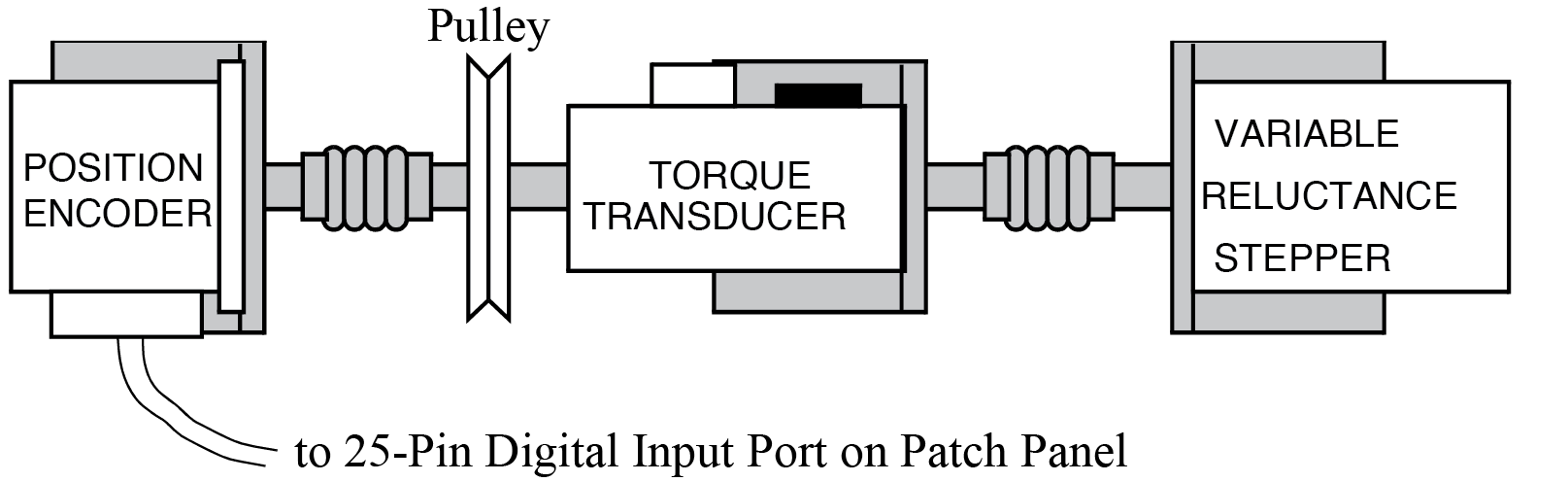
_images/fig12.png — Fig. 5.1 Setup for lab Variable Reluctance Stepper Motor (A).#

5.3.1. Measuring Number of Rotor Teeth#

Ensure that the rotor of the stepper motor is connected to the position encoder through the torque transducer and the cable from the position encoder to the 25-pin Digital Input port of the Patch Panel as shown in Fig. 5.1.
Open the model lab5_tgt.slx. The main window should look similar to Fig. 5.2. The switches are actuated by a mouse double-click. Set the To_IP_Address to the IP number to the host computer on your station.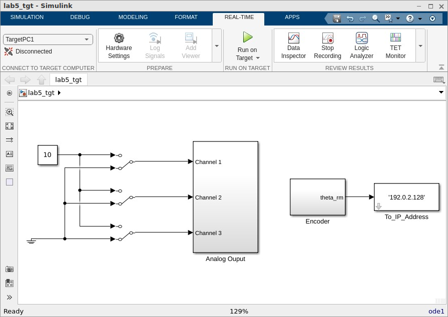

Fig. 5.2 Simulink target model lab5_tgt.slx for measuring step length.#
From REAL-TIME tab, connect to target on your station and press Run on Target.
Open the Simulink model lab5_host.slx, which reads the position transducer in radians. The main window should look similar to Fig. 5.3. Set the FromAddress to the IP number of the target computer at your station. The model is configured as a Normal simulation with the simulation parameters set to Variable-Step with inf as the Stop time. This model runs on the host computer, so it should not be compiled/built.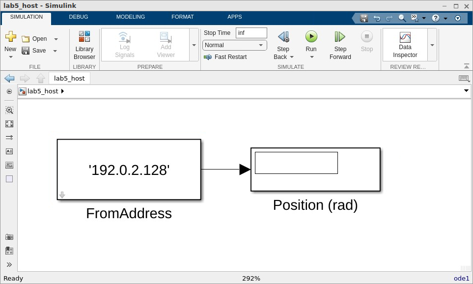

Fig. 5.3 Simulink host PC model lab5_host.slx for measuring step length.#
Apply the \(10\)-\(\volt\) DC signal to the phase-\(a\) winding by clicking in the manual switch in the lab5_tgt window. In the lab5_host window, press Run. Allow the rotor to settle out to its equilibrium position. Record the position of the rotor from the numeric display. Rotate the rotor by hand in either the CW or CCW direction and let it settle to its closest neighboring equilibrium position. Continue turning and stopping the rotor until it has made a full revolution. How many equilibrium points are there in one motor revolution? From this information, how many rotor teeth does the motor possess?

5.3.2. Measuring Step Length#

Record the position of the rotor. Without disturbing the rotor, turn off the DC signal to the phase-\(a\) winding and then energize the phase-\(b\) winding and allow the rotor to settle to its equilibrium position. Turn off phase \(b\) and turn on phase \(c\). Continue manually stepping the phase voltages through the \(a\)-\(b\)-\(c\) \(\cdots\) sequence until the motor has made one full revolution. Record the number of steps required to complete a full revolution. From this, calculate the step length (degrees per step) and verify (5.8).

5.3.3. Measuring DC Resistance#

Measure the DC resistance of the stator winding by applying a DC voltage to one of the windings and measuring the resulting current. Record this value for use in the postlab. When complete, stop the host simulation, then stop the target and disconnect from the target.

5.3.4. Measuring Inductance-Versus-Position#

This procedure requires the use of the prebuilt target-based Simulink model L_vs_pos_tgt.slx, and the host-based Simulink model L_vs_pos_host.slx. The top-level view of L_vs_pos_tgt.slx is shown in Fig. 5.4. This model generates a \(5\)-\(\volt\) \(20\)-\(\hertz\) sinusoidal voltage that is to be applied to one phase of the stepper motor. The voltage-output signal of the power amplifier will be used to measure the phase voltage, and the current-output signal of the power amplifier will be used to measure the corresponding phase current. The voltage-output signal should be connected to Analog Input Channel 1 with the gain knob set to \(10\). The current-output signal should be connected to Analog Input Channel 2 with the gain knob of that input channel set to \(1\). The measured voltage and current signals along with the \(20\)-\(\hertz\) sine and cosine signals are supplied to a block that calculates the inductance at selected rotor positions. This block is described in Appendix A: Measuring Inductance Versus Position. The calculated inductance and measured rotor position are then supplied to the host model L_vs_pos_host.slx. The top level view of L_vs_pos_host.slx is shown in Fig. 5.5. Therein, the numerical values of the measured position and calculated inductance will be displayed in numeric display blocks.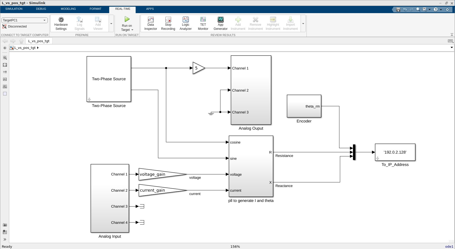

Fig. 5.4 Top-level view of L_vs_pos_tgt.slx.#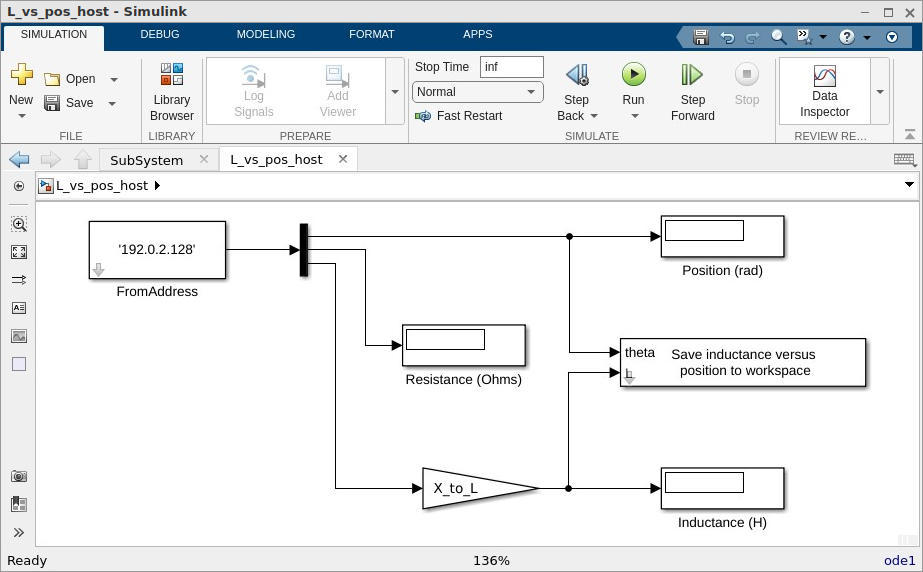

Fig. 5.5 Top-level view of L_vs_pos_host.slx.#
Open L_vs_pos_tgt.slx. Build, connect to target, and start this model. Excite the phase-\(a\) winding with the AC voltage from Channel 1. Connect stepper motor phase \(a\) to Analog Output 1. Remove the connections to the Analog Output 2 and Analog Output 3. Connect the voltage signal from Analog Output 1 to Analog Input 1, and connect the current signal from Analog Output 1 to Analog Input 2. Set the range of Analog Input 1 to \(10\), and the range of Analog Input 2 to \(1\) (middle position). Allow the motor to settle to a stable equilibrium position.

Open L_vs_pos_host.slx and Run to begin the host simulation. This simulation is configured as a Normal simulation. This host model samples the selected signals in the target code L_vs_pos_tgt.slx and displays the measured values in numerical display blocks. Using both hands, rotate the motor rotor slowly and smoothly. Choose and record the direction of rotation (either CW or CCW) when looking from the motor toward the torque transducer. As the rotor rotates, the computer calculates a new value of inductance for each rotor position and updates the digital displays in the host model. After rotating the rotor through one complete revolution, stop the host simulation. In the MATLAB command window, type plot(position, inductance) to verify that the position and inductance data have been written to the MATLAB workspace. Use the following MATLAB command to save the inductance-versus-position data:
```
stepind ('la.mat', position, inductance)
```
The resulting data file la.mat can be used for subsequent plotting and analysis using MATLAB.
Disconnect the \(a\)-phase from Analog Output 1 and connect the \(b\)-phase to Analog Output 1. Restart the host simulation. Measure the inductance versus position of the phase \(b\) winding as done with the \(a\) winding, being sure to rotate the rotor in the same direction as before. Again, save the data in file lb.mat. Repeat the previous steps for the phase \(c\) winding, saving the data in lc.mat. Load la.mat into MATLAB with the command load la.mat in your plotting script. The data will be stored as 2-column matrices of position (radians) and inductance (Henries). Separate the data into vectors of inductance and position, i.e.
```
qrma = position
las = inductance
```
After separating the data, repeat these MATLAB commands for phases \(b\) and \(c\) by loading lb.mat and lc.mat, substituting the appropriate letter for the a in qrma and las. Plot the three inductance curves on one axis, and add appropriate labels.
```
plot(qrma, las, qrmb, lbs, qrmc, lcs)
```
Print the results and save your MATLAB workspace by typing save lab5_ind. Send the file lab5_ind.mat and the provided file fit8.m to a zipped folder and E-mail them to your partner. You will need these files to complete the post lab.

5.4. Postlab#

Use the provided function fit8.m (described in Appendix B: Fitting Parameters to Measured Data) to fit a sinusoidal function to the measured inductance-versus-position data. Express each of the phase inductances in the form

(5.10)#\[L = L_A + L_C \cos RT\theta_{rm} + L_S \sin RT\theta_{rm}\]

where \(L_A\), \(L_C\), and \(L_S\) are contained in the output of fit8.m.
Using the calculated values of \(L_A\), \(L_C\), and \(L_S\), generate arrays of data for the fitted inductance-versus-position characteristics. Plot \(L_{asas}\) versus \(\theta_{rm}\) for both the fitted and measured data, e.g.
```
lascurvefit = L_A + L_C*cos(RT*qrma) + L_S*sin(RT*qrma)
plot(qrma, las, qrma, lascurvefit)
```
Repeat the previous steps for the phase-\(b\) and phase-\(c\) windings. Compare the measured and fitted data. Provide possible explanations for any differences.
On the basis of the fitted inductance-versus-position characteristics, calculate and plot the predicted torque-versus-position for one-phase-on-at-a-time excitation. Specifically, based upon (5.10), calculate coenergy and then \(T_e\) assuming \(I_{as} = 10/r_s\) and \(I_{bs} = I_{cs} = 0\). Repeat the torque-versus-position calculations for phase-\(b\) and phase-\(c\) windings individually. Store the calculated torques in vectors Teacalc, Tebcalc, and Teccalc. You will need these plots to complete Section 6.4, so retain your M-file and check your torque plots with your TA during the next lab session.

5.5. Appendix A: Measuring Inductance Versus Position#

In order to establish the winding inductance, we apply a \(20\)-\(\hertz\) voltage to the winding, i.e.

\[v = 5 \cos(40 \pi t)\]

In phasor form1

\[\tilde{V} = 5\enclose{phasorangle}{0}\]

The measured signal can be expressed in the following general form

(5.11)#\[f = A_f \cos 40 \pi t + B_f \sin 40 \pi t\]

where \(f\) can be substituted for \(v\) or \(i\). It is important to measure \(v\), since the voltage applied may not match the voltage measured. To establish \(A\), we multiply the measured current waveform by \(\cos 40 \pi t\) and average the resulting signal over a period, i.e.

(5.12)#\[A_f = \frac{2}{T} \int_{t - T}^t f(\tau) \cos 40 \pi \tau d\tau \]

This formula can be verified by substituting (5.11) into (5.12) and using the identities

\[\cos x \cos y = \frac{1}{2}\left| 1 - \cos(x + y) \right|\]

\[\cos x \sin y = \frac{1}{2} \cos(x + y)\]

Likewise,

(5.13)#\[B_f = \frac{2}{T} \int_{t - T}^t f(\tau )\sin 40\pi \tau d\tau\]

Given \(A_i\) and \(B_i\), the current phasor can be expressed

\[\tilde{I} = A_i - jB_i\]

and the voltage phasor can be expressed

\[\tilde{V} = A_v - jB_v\]

The impedance of the winding can be calculated as \(Z = \tilde{V} / \tilde{I}\). The resistance and reactance correspond to the real and imaginary components of \(Z\), i.e.

\[R = {\rm Real}(Z) = \frac{A_v A_i + B_v B_i}{A_i^2 + B_i^2}\]

\[X = {\rm Imag}(Z) = \frac{A_v B_i - A_i B_v}{A_i^2 + B_i^2}\]

Finally, the inductance can be established from the reactance as

\[L = \frac{X}{40 \pi}\]

A Simulink model that implements the previous procedure is shown in Fig. 5.6. Therein, the blocks labeled maf implement (5.12) and (5.13). The resistance and reactance, along with the encoder position are sampled by the host model, which is responsible for plotting and storing the results.

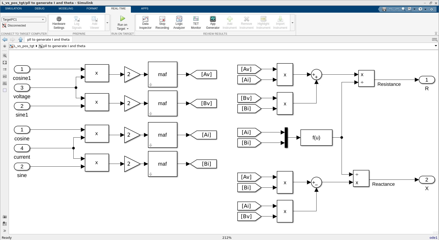
_images/L_vs_pos_tgt_RL_calc.png — Fig. 5.6 Simulink subsystem block that calculates resistance and reactance.#

5.6. Appendix B: Fitting Parameters to Measured Data#

It is assumed that the inductance can be expressed in terms of position as

(5.14)#\[L_s = L_A + L_C \cos{8 \theta_{rm}} + L_S \sin{8 \theta_{rm}}\]

In the lab, we measured an array of inductances and a corresponding array of positions. Substituting the measured inductances and positions into (5.14) results in the following over-specified system of equations.

(5.15)#\[\begin{split}\left[ \begin{array}{ccc} 1 & \cos 8{\theta _1} & \sin 8{\theta _1} \\ 1 & \cos 8{\theta _2} & \sin 8{\theta _2} \\ \cdots & \cdots & \cdots \\ 1 & \cos 8{\theta _N} & \sin 8{\theta _N} \end{array} \right]_{N \times 3} \left[ \begin{array}{c} L_A \\ L_C \\ L_S \end{array} \right] = \left[ \begin{array}{c} L_{1m} \\ L_{2m} \\ \cdots \\ L_{Nm} \end{array} \right]_{N \times 1}\end{split}\]

Here, \(N\) is the number of data points. This set of equations is called over-specified since there are more equations (\(N\)) than unknowns (\(L_A\), \(L_C\), and \(L_S\)). Symbolically, (5.15) can be expressed

(5.16)#\[\mathbf{Ax} = \mathbf{b}\]

where \(\mathbf{x}\) is a vector of unknown parameters, while \(\mathbf{A}\) and \(\mathbf{b}\) are known. Since (5.15) only approximates the inductance-versus-position characteristics, (5.16) is not exact. Denote the error as \(\mathbf{e}\). Equation (5.16) can be rewritten as

(5.17)#\[\mathbf{Ax} - \mathbf{b} = \mathbf{e}\]

The objective is to find \({\mathbf{x}}\) such that

(5.18)#\[\left\| \mathbf{e} \right\|^2 = e_1^2 + e_2^2 + \cdots e_N^2 = \mathbf{e}^T\mathbf{e}\]

is minimized. Substituting (5.17) into (5.18) yields

(5.19)#\[\left\| \mathbf{e} \right\|^2 = \left( \mathbf{Ax} - \mathbf{b} \right)^T \left( \mathbf{Ax} - \mathbf{b} \right) = \mathbf{x}^T \mathbf{A}^T \mathbf{Ax} - \mathbf{x}^T \mathbf{A}^T \mathbf{b} - \mathbf{b}^T \mathbf{Ax} + \mathbf{b}^T \mathbf{b}\]

(5.20)#\[\left\| \mathbf{e} \right\|^2 = \mathbf{x}^T \mathbf{A}^T \mathbf{Ax} - 2 \mathbf{x}^T \mathbf{A}^T \mathbf{b} + \mathbf{b}^T\mathbf{b}\]

Since \(\mathbf{b}^T \mathbf{b}\) is constant, it suffices to minimize the following scalar-valued function

(5.21)#\[f(\mathbf{x}) = \mathbf{x}^T \mathbf{A}^T \mathbf{Ax} - 2 \mathbf{x}^T \mathbf{A}^T \mathbf{b}\]

with respect to \(\mathbf{x}\) where \(\mathbf{Q} = \mathbf{A}^T \mathbf{A}\) and \(\mathbf{y} = \mathbf{A}^T\mathbf{b}\) . To minimize (5.21) with respect to \(\mathbf{x}\), we differentiate with respect to \(\mathbf{x}\) and set the result to zero. With a little work, it can be shown that this procedure results in the matrix equation

(5.22)#\[\mathbf{Qx} = \mathbf{y}\]

Here, \(\mathbf{Q}\) is a nonsingular square matrix (\(3 \times 3\)). Thus, there exists a unique solution \(\mathbf{x}\) that is established by solving (5.22). A simple MATLAB script that evaluates the vector of unknown parameters is given below.

function x = fit8(las, theta)
    for i = 1:length(las)
        A(i,1) = 1;
        A(i,2) = cos(8*theta(i));
        A(i,3) = sin(8*theta(i));
    end
    Q = A'*A;
    y = A'*las;
    x = Q\y; % solve Q*x = y for x

1: Unlike the EE321 text, we will assume the magnitude of the phasor corresponds to the peak (not RMS) amplitude of the corresponding sinusoid.