\[ \begin{align}\begin{aligned}\newcommand\blank{~\underline{\hspace{1.2cm}}~} \newcommand\phase[1]{\enclose{phasorangle}{#1}} \newcommand\RE{\mathrm{Re}} \newcommand\IM{\mathrm{Im}}\\% Bold symbols (vectors) \newcommand\bs[1]{\mathbf{#1}}\\% Poor man's siunitx \newcommand\unit[1]{\mathrm{#1}} \newcommand\num[1]{#1} \newcommand\qty[2]{#1~\unit{#2}}\\\newcommand\per{/} \newcommand\squared{{}^2} % % Scale \newcommand\milli{\unit{m}} \newcommand\kilo{\unit{k}} \newcommand\mega{\unit{M}} % % Angle \newcommand\radian{\unit{rad}} \newcommand\degree{\unit{\kern{-0.5ex}{}^\circ}} % % Time \newcommand\second{\unit{s}} % % Distance \newcommand\meter{\unit{m}} \newcommand\m{\meter} \newcommand\inch{\unit{in}} % % Mass \newcommand\gram{\unit{g}} \newcommand\g{\gram} % % Frequency \newcommand\hertz{\unit{Hz}} \newcommand\rpm{\unit{rpm}} % % Voltage \newcommand\volt{\unit{V}} \newcommand\V{\volt} \newcommand\millivolt{\milli\volt} \newcommand\mV{\milli\volt} \newcommand\kilovolt{\kilo\volt} \newcommand\kV{\kilo\volt} % % Current \newcommand\ampere{\unit{A}} \newcommand\A{\ampere} \newcommand\milliampereA{\milli\ampere} \newcommand\mA{\milli\ampere} \newcommand\kiloampereA{\kilo\ampere} \newcommand\kA{\kilo\ampere} % % Resistance \newcommand\ohm{\Omega} \newcommand\milliohm{\milli\ohm} \newcommand\kiloohm{\kilo\ohm} % correct SI spelling \newcommand\kilohm{\kilo\ohm} % "American" spelling used in siunitx \newcommand\megaohm{\mega\ohm} % correct SI spelling \newcommand\megohm{\mega\ohm} % "American" spelling used in siunitx % % Inductance \newcommand\henry{\unit{H}} \newcommand\H{\henry} \newcommand\millihenry{\milli\henry} \newcommand\mH{\milli\henry} % % Power \newcommand\watt{\unit{W}} \newcommand\W{\watt} \newcommand\milliwatt{\milli\watt} \newcommand\mW{\milli\watt} \newcommand\kilowatt{\kilo\watt} \newcommand\kW{\kilo\watt} % % Torque \newcommand\ozin{\unit{oz}\text{-}\unit{in}} \newcommand\newtonmeter{\unit{N\text{-}m}}\end{aligned}\end{align} \]

8. DC Motor (B)

Objective

The purpose of this experiment is to investigate the characteristics of a permanent-magnet DC motor. The fundamental parameters of a DC motor will be measured whereupon the motor’s steady-state and dynamic operating characteristics will be predicted analytically and by computer simulation. The analytical (closed form) and computer-simulated results will be compared with experimental measurements.

8.1. Prelab

In the previous lab, it was assumed that the torque due to friction could be described using a simple constant \(B_m\) times rotor speed \(\omega_r\). The measured frictional torque vs. rotor speed plot shows that this is not a reasonable assumption, since the slope of the measured data is significantly larger at low rotor speed than at high rotor speed. A better way to model the torque due to friction might be to have an affine rather than linear function to describe torque due to friction, such as:

(8.1)\[T_{\rm friction} = B_m \omega_r + T_{\rm stick}\]

where \(T_{\rm stick}\) is the “sticktion” torque which opposes rotation at low speed.

Using your measured frictional torque versus rotor speed data, re-establish \(B_m\) and find \(T_{\rm stick}\). To do this, determine the average slope and y-intercept of the measured data when rotor speed is greater than zero.

Assuming \(L_{AA}\) can be neglected, the equations of a permanent-magnet DC machine may be expressed:

(8.2)\[k_T i_a = J \frac{d\omega_r}{dt} + B_m \omega_r + T_{\rm stick}\]

(8.3)\[v_a = r_a i_a + k_v \omega_r\]

Starting with equations (8.2) and (8.3), show that by including \(T_{\rm stick}\) in our model, the effective voltage applied to the motor is smaller than we might predict. That is, substitute the motor voltage equation and re-arrange the differential equation to relate \(v_a\) to \(\omega_r\) and show that a constant times \(T_{\rm stick}\) is subtracted from \(v_a\).

8.2. In the Laboratory:

Attention

Safety glasses must be worn at all times during this lab.

8.2.1. Measured torque versus speed

1. Use the same mechanical setup shown in Fig. 8.1. Implement a Simulink model to apply \(\qty{+4}{\V}\) (DC) to the armature of Motor 1 (red with respect to black) at panel output Channel 1 and to apply \(\qty{-4}{\V}\) (DC) to the armature of Motor 2 (red with respect to black) at panel output Channel 2. Both motors should turn with the torque reading near zero.

   

   Fig. 8.1 Configuration for measuring torque vs speed.

2. Measure the current supplied to Motor 1 (test motor) on oscilloscope Channel 1. Measure the tachometer speed on Channel 2, and the torque transducer output voltage on Channel 3. Repeat and record the measurements by varying the Motor 2 voltage from \(\qty{-4}{\V}\) to \(\qty{+4}{\V}\) in \(1\)-\(\V\) steps. Calculate the rotor speed in \(\radian\per\second\), and the torque in \(\newtonmeter\).

8.2.2. Dynamic response

Our objective in this section will be to measure the actual step response with the oscilloscope. We will then establish the motor transient response using a Simulink simulation based on measured parameters and compare results.

Experimental Data

1. Using a Simulink model shown in Fig. 8.2, apply a \(0\) to \(4\)-\(\V\) step to the armature of the DC motor.

   

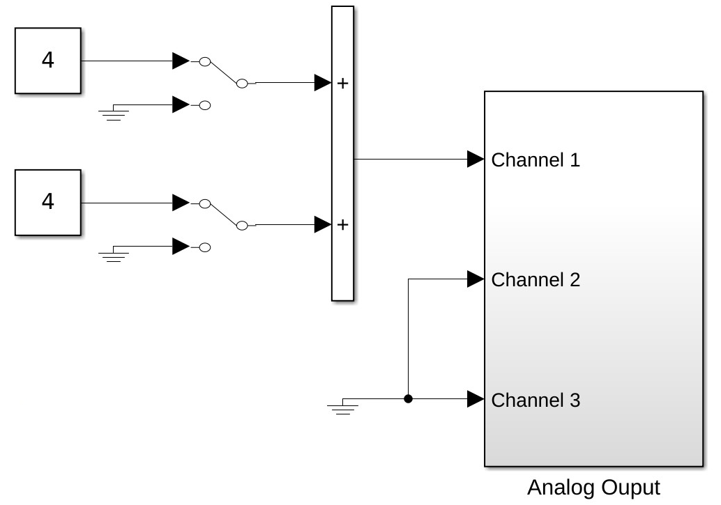
   Fig. 8.2 Simulink model for measuring startup transients (step_transient.slx).

2. Measure the transient armature current on Channel 3 and tachometer voltage (speed) on Channel 2 using the digital oscilloscope. Measure the armature voltage on Channel 1 and set the trigger input to Channel 1 as well. Use single-trigger mode to capture the turn-on transient. Using BenchVue, save the data displayed to a .mat file in your Lab 8 directory. Find the steady-state value and time constant of the exponential response by executing the following command:

   [wrss04,tau04] = fit_wr([75,0.1]',time,wr) 
   

   where time and wr are from the measured data file. This function executes a nonlinear least-squares curve-fitting routine, and can be found in your Lab Lab 8 folder. Using your value for \(\tau_m\), determine the rotor moment of inertia, \(J\).

3. Repeat the experiment for a voltage step from \(\qty{4}{\V}\) to \(\qty{8}{\V}\). Save the data into a new .mat file, and re-establish the steady-state rotor speed, mechanical time constant, and rotor moment of inertia. The rotor has already developed a speed in this test, so the previous value of steady-state speed must be subtracted before executing the curve-fitting for the algorithm to work. The data can be shifted back after the program has finished. To do this, execute the following commands:

   [wrss48_shifted,tau48] = fit_wr([75,0.1]',time,wr-wrss04)
   wrss48 = wrss48_shifted + wrss04
   

4. How do the values from the \(\qty{4}{\V}\) to \(\qty{8}{\V}\) step differ from the values from the \(\qty{0}{\V}\) to \(\qty{4}{\V}\) step, and by how much do they differ? What are potential reasons for any differences?

Computer Simulation

1. Simulate the startup characteristics using the electrical and mechanical parameters measured in the lab. A Simulink program, motorsim1.slx, is available to perform this simulation. The simulation program is shown below. Enter the motor parameters by double-clicking on the DC Motor Dynamics block. Generate a printout of the simulated response of a \(\qty{0}{\V}\) to \(\qty{4}{\V}\) step input. Also, record the electrical and mechanical parameters that were used to generate the plots, measure simulated time constant (for use in postlab), and final speed. Be sure to use your own parameters and not those shown in Figure 3.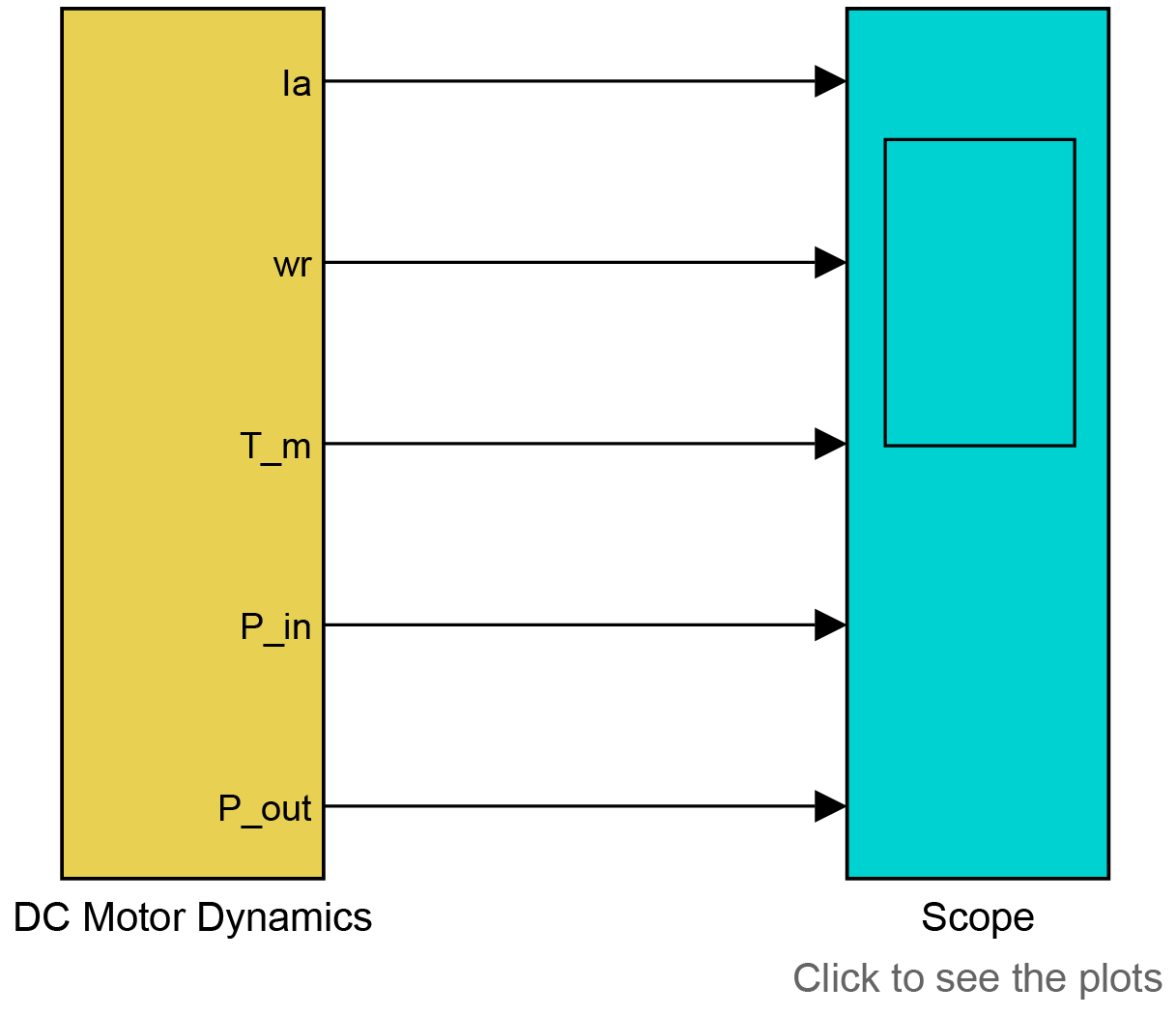

   

   Fig. 8.3 Top layer and dialog box for Simulink model motorsim1.slx.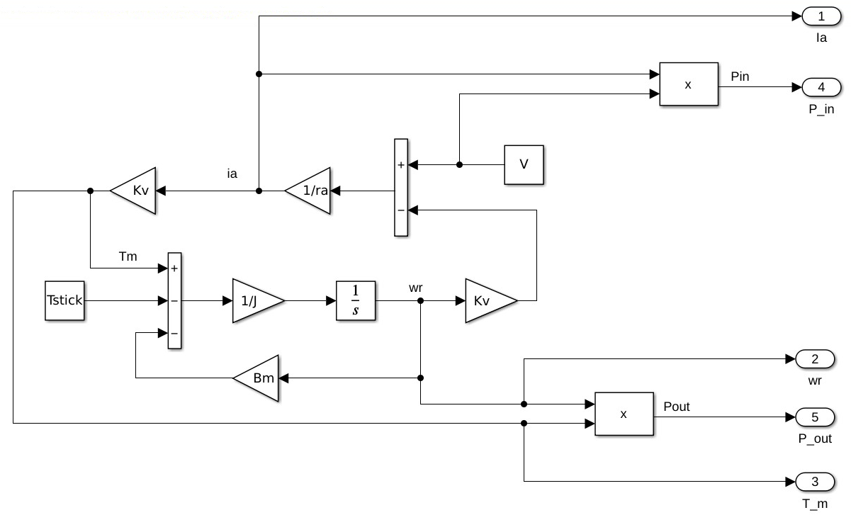

   

   Fig. 8.4 Simulink model DC motor dynamics block.

8.3. Postlab

1. Plot the measured torque versus speed and the predicted characteristics from Experiment 7.3 Postlab on the same axis and compare the results.

2. Why is it reasonable to neglect \(L_{AA}\)?

3. Using Matlab, implement the closed-form equation of \(\omega_r(t)\) derived in last week’s prelab, generate a plot of \(\omega_r\) versus time for a \(\qty{0}{\V}\) to \(\qty{4}{\V}\) step input. Record the parameters (\(k_T\), \(k_v\), \(r_a\), and \(B_m\)) used to generate this plot.

4. What were some differences between the measured rotor speed response to the \(\qty{0}{\V}\) to \(\qty{4}{\V}\) input versus the \(\qty{4}{\V}\) to \(\qty{8}{\V}\) input? What do you think caused the differences?

5. How closely did the experimental and simulated \(\omega_r(t)\) curves match (consider the difference in the time constant and final speed). What are some possible explanations for the differences between the predicted and measured curves?

6. Why do we use a tachometer instead of armature terminal voltage to measure the rotor speed?

7. Which measure (an encoder or a tachometer) is more accurate? In what situations are a tachometer more desirable than an encoder? In what situations are an encoder more desirable than a tachometer?

   Note

   The encoder is a digital device used in previous labs to measure rotor position.