\[ \begin{align}\begin{aligned}\newcommand\blank{~\underline{\hspace{1.2cm}}~} \newcommand\phase[1]{\enclose{phasorangle}{#1}} \newcommand\RE{\mathrm{Re}} \newcommand\IM{\mathrm{Im}}\\% Bold symbols (vectors) \newcommand\bs[1]{\mathbf{#1}}\\% Poor man's siunitx \newcommand\unit[1]{\mathrm{#1}} \newcommand\num[1]{#1} \newcommand\qty[2]{#1~\unit{#2}}\\\newcommand\per{/} \newcommand\squared{{}^2} % % Scale \newcommand\milli{\unit{m}} \newcommand\kilo{\unit{k}} \newcommand\mega{\unit{M}} % % Angle \newcommand\radian{\unit{rad}} \newcommand\degree{\unit{\kern{-0.5ex}{}^\circ}} % % Time \newcommand\second{\unit{s}} % % Distance \newcommand\meter{\unit{m}} \newcommand\m{\meter} \newcommand\inch{\unit{in}} % % Mass \newcommand\gram{\unit{g}} \newcommand\g{\gram} % % Frequency \newcommand\hertz{\unit{Hz}} \newcommand\rpm{\unit{rpm}} % % Voltage \newcommand\volt{\unit{V}} \newcommand\V{\volt} \newcommand\millivolt{\milli\volt} \newcommand\mV{\milli\volt} \newcommand\kilovolt{\kilo\volt} \newcommand\kV{\kilo\volt} % % Current \newcommand\ampere{\unit{A}} \newcommand\A{\ampere} \newcommand\milliampereA{\milli\ampere} \newcommand\mA{\milli\ampere} \newcommand\kiloampereA{\kilo\ampere} \newcommand\kA{\kilo\ampere} % % Resistance \newcommand\ohm{\Omega} \newcommand\milliohm{\milli\ohm} \newcommand\kiloohm{\kilo\ohm} % correct SI spelling \newcommand\kilohm{\kilo\ohm} % "American" spelling used in siunitx \newcommand\megaohm{\mega\ohm} % correct SI spelling \newcommand\megohm{\mega\ohm} % "American" spelling used in siunitx % % Inductance \newcommand\henry{\unit{H}} \newcommand\H{\henry} \newcommand\millihenry{\milli\henry} \newcommand\mH{\milli\henry} % % Power \newcommand\watt{\unit{W}} \newcommand\W{\watt} \newcommand\milliwatt{\milli\watt} \newcommand\mW{\milli\watt} \newcommand\kilowatt{\kilo\watt} \newcommand\kW{\kilo\watt} % % Torque \newcommand\ozin{\unit{oz}\text{-}\unit{in}} \newcommand\newtonmeter{\unit{N\text{-}m}}\end{aligned}\end{align} \]

4. Electromagnetic Forces (B)

Objective

The objective of this experiment is to study the interaction between electrical and mechanical systems that are coupled magnetically. The electromechanical relay (solenoid) studied in Experiment 2 will be analyzed to predict its steady-state force-versus-position and force-versus-current characteristics. Moreover, computer simulation will be used to predict its dynamic force-versus-time characteristics. The analytical and simulated results will be compared with laboratory measurements.

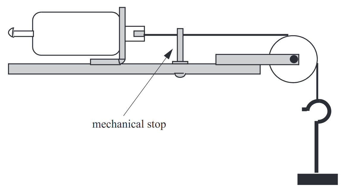
Fig. 4.1 Setup for Experiment 4.

4.1. Introduction:

In this lab, we will consider the cylindrical solenoid depicted in Fig. 4.2. In the previous experiment, it was shown that the self-inductance can be approximated as

(4.1)\[L(x) = L_l + \frac{K}{k_0+x}\]

Here, \(K\) and \(k_0\) are assumed to be known constants and \(L_l\) is the leakage inductance. In the prelab, we will establish an expression for force versus position and express the electrical and mechanical equations in state-space form.

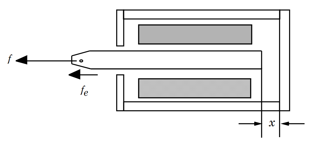
Fig. 4.2 Simplified cross-sectional view of cylindrical solenoid.

Hopefully, our experimental measurements will confirm the general form of this equation.

4.2. Prelab

Let \(M\) denote the mass of the plunger and \(f\) the externally applied force (Fig. 4.2). Newton’s law of motion may be expressed.

(4.2)\[f + f_e(i,x) = M\frac{d^2x}{dt^2}\]

This second-order differential equation may be expressed as two first-order equations

(4.3)\[\frac{dv_x}{dt}=\frac{1}{M}\left[ f_e(i,x)+f\right]\]

(4.4)\[\frac{dx}{dt} = v_x\]

where \(v_x\) is the velocity, \(x\) is the position, \(i\) is the current, \(v\) is the applied voltage and \(f\) is the externally applied force. The electrical equation may be expressed symbolically as

(4.5)\[\frac{d\lambda}{dt} = g(\lambda,v,x)\]

where \(g\) is a function of the indicated arguments.

Starting with \(\displaystyle v = ri + \frac{d \lambda}{dt}\) and \(\lambda = L(x)i\), derive an expression for \(g\) in terms of \(\lambda\), \(v\), and \(x\). Equations (4.3)-(4.5) represent the state equations of the electromechanical system where \(v_x\) and \(x\), and are state variables, while \(v\) and \(f\) are inputs. The parameters are \(K\), \(k_0\), and \(r\) (coil resistance).

The three coupled first-order differential equations contain nonlinear terms and are therefore difficult to solve analytically. A technique that can be used to solve the differential equations numerically is outlined below. A Simulink model of the solenoid is shown in Fig. 4.3. This model is based upon the equations set forth in (4.2)-(4.5). Additional logic is provided to prevent the solenoid position from becoming negative (an impossibility, at least in classic Physics). In particular, when \(x\) tries to go negative, the output Q of the SR flip-flop is set high, which, in turn, sets and holds the integrator that calculates \(v_x\) to zero. When the net applied force is greater than zero, the flip-flop is reset, which “releases” the integrator that calculates \(v_x\) (allowing \(v_x\) to become positive).

Look at this Simulink model and compare with the equations found in prelabs 3.2 and 4.2 Be prepared to take a quiz on these equations based with respect to electromagnetic and electromechanical force at the beginning of the lab period.

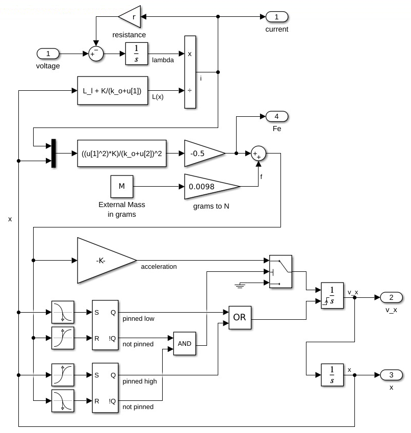
Fig. 4.3 Simulink model of solenoid.

4.3. In the Laboratory:

Try to resolve gross discrepancies between measured and calculated plots by repeating necessary measurements. Identify the discrepancies encountered. Our final objective will be to investigate the solenoid dynamics.

4.3.1. Solenoid Dynamics

1. Execute the program proj3.mdl that should be in the Lab 4 directory. This opens a Simulink project window.

2. Simulate the solenoid pull-in characteristics for each combination of \(x_0\) at \(\qty{1/8}{\inch}\) and \(\qty{3/8}{\inch}\) and \(M\) at \(0\), \(50\), \(100\), and \(\qty{150}{\g}\). In proj3.mdl, \(M\) is the external mass. The plunger mass is \(\qty{35}{\g}\). Double-click the Subsystem block to open a dialog window and fill in the parameters (\(x_0\), \(M\), \(r\), \(L_l\), \(K\), and \(k_0\)). Right-selecting the block in the Simulink project window and choosing Look Under Mask opens a second window that displays the model shown in Fig. 4.3. Run the model as a normal Simulink model (that is, do not build a target model). Record the time for the plunger to reach \(x=0\). Make printouts of the waveforms for the (\(\qty{1/8}{\inch}\), \(\qty{150}{\g}\)), and (\(\qty{3/8}{\inch}\), \(\qty{0}{\g}\)) simulations.

4.3.2. Measuring Plunger Pull-In Time

Remove the weights from the solenoid plunger. Position the plunger at \(\qty{1/8}{\inch}\) using the set screw for calibration. Position the mechanical stop (Fig. 4.1) so that \(x\) cannot exceed \(\qty{1/8}{\inch}\). Then, remove the set screw. Apply a \(12\)-\(\volt\) step to the solenoid coil. The solenoid should “pull in”. Set the oscilloscope to single-sweep mode and set the timescale to \(\qty{20}{\milli\second\per div}\). Capture the measured current waveform as the solenoid “pulls in”. You will with near certainty have to repeat this step several times to capture the desired data.

Measure the time from application of the step voltage to the “dip” in the current waveform using paired cursors.

Add \(50\), \(100\), and \(\qty{150}{\g}\) weights to the solenoid plunger and repeat the pull-in time measurements. Use BenchVue to get and print a snapshot of the \(\qty{1/8}{\inch}\), \(\qty{150}{\g}\) response showing the paired cursor measurement.

Repeat the transition time measurements using a starting position of \(\qty{3/8}{\inch}\). Using BenchVue, capture and print the simulated and measured current-versus-time data for the \(\qty{3/8}{\inch}\), \(\qty{0}{\g}\) trial. Explain the discrepancies between the simulated and experimental results.

Table 4.1 Pull-in Time Data

\(x_0\) (\(\inch\))	Mass (\(\g\))	Simulated Pull-in Time (\(\milli\second\))	Measured Pull-in Time (\(\milli\second\))
\(1/8\)	\(0\)
	\(50\)
	\(100\)
	\(150\)
\(3/8\)	\(0\)
	\(50\)
	\(100\)
	\(150\)

4.4. Postlab

1. Provide an explanation for the “dip” in solenoid current when the plunger pulls in.

   Hint

   (4.6)\[v = ri + \frac{d}{dt}[L(x)i] = ri + L(x) \frac{di}{dt} + \frac{dL(x)}{dx}\frac{dx}{dt}\]

   How do \(L(x)\), \(\displaystyle\frac{dL}{dx}\), and \(\displaystyle\frac{dx}{dt}\) vary during the pull-in transient?

Use relevant equations to provide answers to the following questions:

2. Why does solenoid inductance decrease as the plunger position increases?

3. Why does the solenoid force decrease as the plunger position increases?

4. What is the relationship between force and current? What is the relationship between force and position?

5. What happens to the plunger if the solenoid coil polarity is reversed?

6. Can the plunger be made to “push out” instead of “pull in”? Explain.